Processing sequence for acoustic impedance estimation

Seismic Data Analysis

Series	Investigations in Geophysics
Author	Öz Yilmaz
DOI	http://dx.doi.org/10.1190/1.9781560801580
ISBN	ISBN 978-1-56080-094-1
Store	SEG Online Store

The parsimonious signal processing sequence described in analysis of amplitude variation with offset tailored for AVO analysis also should be used for acoustic impedance estimation. Again, it is important to preserve the signal bandwidth of there-corded data during processing and attain a broad-band spectrum with a flat passband for the data input to poststack amplitude inversion. Also, the processing sequence must be designed to preserve relative amplitudes in the data. We shall analyze a 2-D marine line for acoustic impedance estimation. Data specifications for the line are listed in Table 11-4. In addition to the seismic data, sonic and density logs from a well located on the line traverse were used in estimating and removing the constant and linear phase associated with the residual wavelet in the poststack time-migrated CMP stacked data prior to amplitude inversion.

Table 11-4. Data specifications for the line used in acoustic impedance estimation.

Line Length	23.2 km
Shot Spacing	25 m
Receiver Spacing	16.67 m
CMP Spacing	8.33 m
Minimum Offset	80 m
Maximum Offset	3064 m
Number of Receivers	180
Fold of Coverage	60
Sampling interval	2 ms

The processing sequence included the following steps:

1. Design a Wiener shaping filter (field data examples) to convert the recorded far-field source signature to its minimum-phase equivalent. Then, perform signature deconvolution by applying the filter to the recorded data.
2. Mute guided waves since they are confined to the shallow water layer and contain no information about the subsurface reflectivity.
3. Apply t²-scaling to compensate for geometric spreading. As mentioned in analysis of amplitude variation with offset, a velocity-dependent scaling function should be avoided to prevent overcorrection of amplitudes of multiples.
4. Perform predictive deconvolution with unit-prediction lag to increase the vertical resolution, and remove short-period multiples and reverberations. With increasing prediction lag, the amplitude spectrum departs from a flat character (predictive deconvolution in practice). No data-dependent scaling should be applied to ensure preservation of relative amplitudes.
5. Test CMP stacking for optimum fold (Figure 11.3-3). The principle criterion is to ensure minimal dependency of reflection amplitudes on the angle of incidence within the time window of interest. By using the NMO-corrected CMP gathers at velocity analysis locations, derive a spatially varying mute pattern such that much of the far-offset data are excluded from stacking. The CMP stack with optimum mute (Figure 11.3-3a) appears to best preserve the flatness character of the average amplitude spectrum of the data. The amplitude spectra and the autocorrelograms imply that there needs to be further flattening of the spectrum within the passband and removal of reverberations.
6. Perform velocity analyses at frequent intervals, and obtain an optimum CMP stack using a time- and spatially varying mute function.
7. Apply a frequency-space complex Wiener filter with unit-prediction lag (f − x deconvolution) to attenuate random noise uncorrelated from trace to trace (Figure 11.3-4a).
8. Apply minimum-phase deconvolution to restore flat spectrum within the passband (Figure 11.3-4b).
9. Apply time-variant spectral whitening to account for nonstationarity (Figure 11.3-4c).
10. Design and apply a time-varying filter, while maintaining the broadest possible signal band. Again, any data-dependent scaling must not be applied to preserve relative amplitudes.
11. Migrate the optimum CMP stacked data using a phase-shift algorithm. Migration compensates for the effect of reflector curvature on reflection amplitudes (equation 13a) so that the resulting amplitudes can be related directly to acoustic impedance variations. The reason for using the phase-shift algorithm is that, compared to finite-difference or integral methods, it causes the least phase and amplitude errors. Additionally, amplitude inversion often is applied to data associated with a velocity field that varies very mildly in the lateral direction.

Failed to parse (SVG (MathML can be enabled via browser plugin): Invalid response ("Math extension cannot connect to Restbase.") from server "https://en.wikipedia.org/api/rest_v1/":): CE=\frac{1}{\sqrt{1+A^{-1}z}},

(13a)

Poststack time migration may precede the poststack signal processing, particularly deconvolution. As a result of migration, we transform a 2-D or a 3-D wavefield to a 1-D wavefield along the seismic traverse. Hence, we map the normal-incident energy to vertical-incident energy and obtain 1-D zero-offset seismograms at each CMP location. This satisfies the underlying assumption for poststack deconvolution.

Figure 11.3-5 shows the test panel for poststack processing in which migration precedes the signal processing. The sequence includes f − x deconvolution, phase-shift migration (Figure 11.3-5a), spiking deconvolution (Figure 11.3-5b), time-variant spectral whitening (Figure 11.3-5c), and time-variant filtering (Figure 11.3-5d). Finally, a mild (3-trace) Karhunen-Loeve filter was applied to the data to attenuate coherent linear noise and any remaining random noise uncorrelated from trace to trace (Figure 11.3-5e). The unmigrated CMP stack with the poststack processing as in Figure 11.3-4 is shown in Figure 11.3-6 and the migrated CMP stack with the poststack processing as in Figure 11.3-5 is shown in Figure 11.3-7.

• 
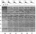  Figure 11.3-3  A portion of a CMP stack for a test for optimum stacking fold using different cable lengths: (a) using an optimum mute pattern that minimizes angle dependency of seismic amplitudes, (b) using a mute pattern that provides a full-offset stack, (c) 75 percent near-offset stack, (d) 50 percent near-offset stack, (e) 25 percent near-offset stack, and (f) 17 percent near-offset stack. On top of each panel is the amplitude spectrum averaged over the shot record, and at the bottom is the autocorrelogram.
• 
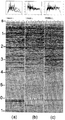  Figure 11.3-4  A portion of the CMP stack as in Figure 11.3-3a after: (a) poststack f − x deconvolution to attenuate random noise, (b) spiking deconvolution, and (c) time-variant spectral whitening. On top of each panel is the amplitude spectrum averaged over the shot record, and at the bottom is the autocorrelogram.
• 
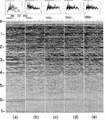  Figure 11.3-5  A portion of the time-migrated CMP stack after: (a) f − x deconvolution, (b) spiking deconvolution, (c) time-variant spectral whitening, (d) time-variant filtering, and (e) Karhunen-Loeve filtering. On top of each panel is the amplitude spectrum averaged over the shot record, and at the bottom is the autocorrelogram.
• 
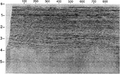  Figure 11.3-6  Unmigrated CMP stack with poststack processing as in Figure 11.3-4.
• 
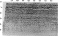  Figure 11.3-7  Migrated CMP stack with poststack processing as in Figure 11.3-5.

Below is a summary of key issues regarding the processing sequence appropriate for amplitude inversion applied to poststack time-migrated CMP data.

1. Avoid f − k filtering. This type of filtering invariably causes amplitude distortions. For multiple attenuation, use predictive deconvolution with a long operator length; the process will be effective at near offsets where periodicity of multiples are nearly preserved.
2. Do not apply a velocity-dependent scaling function to compensate for geometric spreading. The amplitudes of multiples will be overcorrected with a velocity-dependent scaling function. A t²-scaling is favored for data to be used in amplitude inversion.
3. Use the phase-shift method for migration. Differencing approximations to differential operators used in finite-difference migration induce phase errors and cause amplitude distortions. The usual implementation of the Kirchhoff migration (equation H-17, Section H.1) does not include all the terms of the integral solution (equation H-16) to the scalar wave equation. As such, the missing terms can influence the amplitude and phase accuracy of the resulting migrated data.
4. You may be required to apply a harsh mute in stacking. Design a mute function at each velocity analysis location and apply a spatially varying mute pattern to the data for stacking. The design criterion is such that reflection amplitudes should be uniform within the offset range included in the stacking for an event.
5. You may want to migrate before, and not after, poststack deconvolution. This is to conform with the fundamental assumption that deconvolution acts upon a 1-D zero-offset reflection seismogram recorded over a horizontally layered earth model. Amplitudes associated with any phantom diffractions should not be present on the traces input to deconvolution.

See also

• Acoustic impedance estimation
• Synthetic sonic logs
• Derivation of acoustic impedance attribute
• 3-D acoustic impedance estimation
• Instantaneous attributes

External links

find literature about Processing sequence for acoustic impedance estimation