Predictive deconvolution

The type 3 desired output, a time-advanced form of the input series, suggests a prediction process. Given the input x(t), we want to predict its value at some future time (t + α), where α is prediction lag. Wiener showed that the filter used to estimate x(t + α) can be computed by using a special form of the matrix equation (30) . Since the desired output x(t + α) is the time-advanced version of the input x(t), we need to specialize the right side of equation (30) for the prediction problem.

Consider a five-point input time series x(t): (x₀, x₁, x₂, x₃, x₄), and set α = 2. The autocorrelation of the input series is computed in Table 2-23, and the crosscorrelation between the desired output x(t + 2) and the input x(t) is computed in Table 2-24. Compare the results in Tables 2-23 and 2-24, and note that g_i = r_i+α for α = 2 and i = 0, 1, 2, 3, 4.

Equation (30), for this special case, is rewritten as follows:

${\begin{pmatrix}r_{0}&r_{1}&r_{2}&\cdots &r_{n-1}\\r_{1}&r_{0}&r_{1}&\cdots &r_{n-2}\\r_{2}&r_{1}&r_{0}&\cdots &r_{n-3}\\\vdots &\vdots &\vdots &\ddots &\vdots \\r_{n-1}&r_{n-2}&r_{n-3}&\cdots &r_{0}\end{pmatrix}}{\begin{pmatrix}a_{0}\\a_{1}\\a_{2}\\\vdots \\a_{n-1}\\\end{pmatrix}}={\begin{pmatrix}g_{0}\\g_{1}\\g_{2}\\\vdots \\g_{n-1}\end{pmatrix}}$

(30)

${\begin{pmatrix}r_{0}&r_{1}&r_{2}&r_{3}&r_{4}\\r_{1}&r_{0}&r_{1}&r_{2}&r_{3}\\r_{2}&r_{1}&r_{0}&r_{1}&r_{2}\\r_{3}&r_{2}&r_{1}&r_{0}&r_{1}\\r_{4}&r_{3}&r_{2}&r_{1}&r_{0}\\\end{pmatrix}}{\begin{pmatrix}a_{0}\\a_{1}\\a_{2}\\a_{3}\\a_{4}\\\end{pmatrix}}={\begin{pmatrix}r_{2}\\r_{3}\\r_{4}\\r_{5}\\r_{6}\\\end{pmatrix}}.$

(34)

The prediction filter coefficients a(t) : (a₀, a₁, a₂, a₃, a₄) can be computed from equation (34) and applied to the input series x(t) : (x₀, x₁, x₂, x₃, x₄) to compute the actual output y(t) : (y₀, y₁, y₂, y₃, y₄) (Table 2-25). We want to predict the time-advanced form of the input; hence, the actual output is an estimate of the series x(t + α) : (x₂, x₃, x₄), where α = 2. The prediction error series e(t) = x(t + α) − y(t) : (e₂, e₃, e₄, e₅, e₆) is given in Table 2-26.

The results in Table 2-26 suggest that the error series can be obtained more directly by convolving the input series x(t) : (x₀, x₁, x₂, x₃, x₄) with a filter with coefficients (1, 0, −a₀, −a₁, −a₂, −a₃, −a₄) (Table 2-27). The results for (e₂, e₃, e₄, e₅, e₆) are identical (Tables 2-26 and 2-27). Since the series (a₀, a₁, a₂, a₃, a₄) is called the prediction filter, it is natural to call the series (1, 0, −a₀, −a₁, −a₂, −a₃, −a₄) the prediction error filter. When applied to the input series, this filter yields the error series in the prediction process (Table 2-27).

Table 2-23. Autocorrelation lags of input series x(t) : (x₀, x₁, x₂, x₃, x₄).

$r_{0}=x_{0}^{2}+x_{1}^{2}+x_{2}^{2}+x_{3}^{2}+x_{4}^{2}$

r1 = x0x1 + x1x2 + x2x3 + x3x4

r2 = x0x2 + x1x3 + x2x4

r3 = x0x3 + x1x4

r4 = x0x4

r5 = 0

r6 = 0

Table 2-24. Crosscorrelation of desired output x(t + α): (x₂, x₃, x₄), α = 2, with input x(t) : (x₀, x₁, x₂, x₃, x₄)

g0 = x0x2 + x1x3 + x2x4

g1 = x0x3 + x1x4

g2 = x0x4

g3 = 0

g4 = 0

Table 2-25. Convolution of prediction filter a(t): (a₀, a₁, a₂, a₃, a₄) with input series x(t): (x₀, x₁, x₂, x₃, x₄) to compute actual output y(t) : (y₀, y₁, y₂, y₃, y₄).

y0 = a0x0

y1 = a1x0 + a0x1

y2 = a2x0 + a1x1 + a0x2

y3 = a3x0 + a2x1 + a1x2 + a0x3

y4 = a4x0 + a3x1 + a2x2 + a1x3 + a0x4

Table 2-26. The error series e(t) = x(t + α) − y(t) : (e₂, e₃, e₄, e₅, e₆), α = 2. For y(t), see Table 2-25.

e2 = x2 − a0x0

e3 = x3 − a1x0 − a0x1

e4 = x4 − a2x0 − a1x1 − a0x2

e5 = 0 − a3x0 − a2x1 − a1x2 − a0x3

e6 = 0 − a4x0 − a3x1 − a2x2 − a1x3 − a0x4

Table 2-27. Convolution of prediction error filter coefficients (1, 0, −a₀, −a₁, −a₂, −a₃, −a₄) with input series x(t) : (x₀, x₁, x₂, x₃, x₄).

e0 = x0

e1 = x1

e2 = x2 − a0x0

e3 = x3 − a1x0 − a0x1

e4 = x4 − a2x0 − a1x1 − a0x2

e5 = 0 − a3x0 − a2x1 − a1x2 − a0x3

e6 = 0 − a4x0 − a3x1 − a2x2 − a1x3 − a0x4

Why place so much emphasis on the error series? Consider the prediction process as it relates to a seismic trace. From the past values of a time series up to time t, a future value can be predicted at time t + α, where α is the prediction lag. A seismic trace often has a predictable component (multiples) with a periodic rate of occurrence. According to assumption 6, anything else, such as primary reflections, is unpredictable.

Some may claim that reflections are predictable as well; this may be the case if deposition is cyclic. However, this type of deposition is not often encountered. While the prediction filter yields the predictable component (the multiples) of a seismic trace, the remaining unpredictable part, the error series, is essentially the reflection series.

Equation (34) can be generalized for the case of an n-long prediction filter and an α-long prediction lag.

${\begin{pmatrix}r_{0}&r_{1}&r_{2}&\cdots &r_{n-1}\\r_{1}&r_{0}&r_{1}&\cdots &r_{n-2}\\r_{2}&r_{1}&r_{0}&\cdots &r_{n-3}\\\vdots &\vdots &\vdots &\ddots &\vdots \\r_{n-1}&r_{n-2}&r_{n-3}&\cdots &r_{0}\\\end{pmatrix}}{\begin{pmatrix}a_{0}\\a_{1}\\a_{2}\\\vdots \\a_{n-1}\\\end{pmatrix}}={\begin{pmatrix}r_{\alpha }\\r_{\alpha +1}\\r_{\alpha +2}\\\vdots \\r_{\alpha +n-1}\\\end{pmatrix}}$

(35)

Note that design of the prediction filters requires only autocorrelation of the input series.

There are two approaches to predictive deconvolution:

1. The prediction filter (a₀, a₁, a₂, …, a_n−1) may be designed using equation (35) and applied on input series as described in Figure 2.3-10.
2. Alternatively, the prediction error filter (1, 0, 0, …, 0, −a₀, −a₁, −a₂, …, −a_n−1) can be designed and convolved with the input series as described in Figure 2.3-11.

Now consider the special case of unit prediction lag, α = 1. For n = 5, equation (35) takes the following form:

${\begin{pmatrix}r_{0}&r_{1}&r_{2}&r_{3}&r_{4}\\r_{1}&r_{0}&r_{1}&r_{2}&r_{3}\\r_{2}&r_{1}&r_{0}&r_{1}&r_{2}\\r_{3}&r_{2}&r_{1}&r_{0}&r_{1}\\r_{4}&r_{3}&r_{2}&r_{1}&r_{0}\\\end{pmatrix}}{\begin{pmatrix}a_{0}\\a_{1}\\a_{2}\\a_{3}\\a_{4}\\\end{pmatrix}}={\begin{pmatrix}r_{1}\\r_{2}\\r_{3}\\r_{4}\\r_{5}\\\end{pmatrix}}.$

(36)

By augmenting the right side to the left side, we obtain:

${\begin{pmatrix}-r_{1}&r_{0}&r_{1}&r_{2}&r_{3}&r_{4}\\-r_{2}&r_{1}&r_{0}&r_{1}&r_{2}&r_{3}\\-r_{3}&r_{2}&r_{1}&r_{0}&r_{1}&r_{2}\\-r_{4}&r_{3}&r_{2}&r_{1}&r_{0}&r_{1}\\-r_{5}&r_{4}&r_{3}&r_{2}&r_{1}&r_{0}\\\end{pmatrix}}{\begin{pmatrix}1\\a_{0}\\a_{1}\\a_{2}\\a_{3}\\a_{4}\\\end{pmatrix}}={\begin{pmatrix}0\\0\\0\\0\\0\\0\\\end{pmatrix}}.$

(37)

Add one row and move the negative sign to the column matrix that represents the filter coefficients to get:

${\begin{pmatrix}r_{0}&r_{1}&r_{2}&r_{3}&r_{4}&r_{5}\\r_{1}&r_{0}&r_{1}&r_{2}&r_{3}&r_{4}\\r_{2}&r_{1}&r_{0}&r_{1}&r_{2}&r_{3}\\r_{3}&r_{2}&r_{1}&r_{0}&r_{1}&r_{2}\\r_{4}&r_{3}&r_{2}&r_{1}&r_{0}&r_{1}\\r_{5}&r_{4}&r_{3}&r_{2}&r_{1}&r_{0}\\\end{pmatrix}}{\begin{pmatrix}1\\-a_{0}\\-a_{1}\\-a_{2}\\-a_{3}\\-a_{4}\\\end{pmatrix}}={\begin{pmatrix}L\\0\\0\\0\\0\\0\\\end{pmatrix}}.$

(38)

where L = r₀ − r₁a₀ − r₂a₁ − r₃a₂ − r₄a₃ − r₅a₄. Note that there are six unknowns, (a₀, a₁, a₂, a₄, a₅, L), and six equations. Solution of these equations yields the unit-delay prediction error filter (1, −a₀, −a₁, −a₂, −a₄, −a₅), and the quantity L — the error in the filtering process (Section B.5). We can rewrite equation (38) as follows:

${\begin{pmatrix}r_{0}&r_{1}&r_{2}&r_{3}&r_{4}&r_{5}\\r_{1}&r_{0}&r_{1}&r_{2}&r_{3}&r_{4}\\r_{2}&r_{1}&r_{0}&r_{1}&r_{2}&r_{3}\\r_{3}&r_{2}&r_{1}&r_{0}&r_{1}&r_{2}\\r_{4}&r_{3}&r_{2}&r_{1}&r_{0}&r_{1}\\r_{5}&r_{4}&r_{3}&r_{2}&r_{1}&r_{0}\\\end{pmatrix}}{\begin{pmatrix}b_{0}\\b_{1}\\b_{2}\\b_{3}\\b_{4}\\b_{5}\\\end{pmatrix}}={\begin{pmatrix}L\\0\\0\\0\\0\\0\\\end{pmatrix}}.$

(39)

where b₀ = 1, b_i = −a_i, and i = 1, 2, 3, 4, 5. This equation has a familiar structure. In fact, except for the scale factor L, it has the same form as equation (31), which yields the coefficients for the least-squares zero-delay inverse filter. This inverse filter is therefore the same as the prediction error filter with unit prediction lag, except for a scale factor. Hence, spiking deconvolution actually is a special case of predictive deconvolution with unit prediction lag.

${\begin{pmatrix}r_{0}&r_{1}&r_{2}&\cdots &r_{n-1}\\r_{1}&r_{0}&r_{1}&\cdots &r_{n-2}\\r_{2}&r_{1}&r_{0}&\cdots &r_{n-3}\\\vdots &\vdots &\vdots &\ddots &\vdots \\r_{n-1}&r_{n-2}&r_{n-3}&\cdots &r_{0}\end{pmatrix}}{\begin{pmatrix}a_{0}\\a_{1}\\a_{2}\\\vdots \\a_{n-1}\\\end{pmatrix}}={\begin{pmatrix}1\\0\\0\\\vdots \\0\end{pmatrix}}$

(31)

We now know that predictive deconvolution is a general process that encompasses spiking deconvolution. In general, the following statement can be made: Given an input wavelet of length (n + α), the prediction error filter contracts it to an α-long wavelet, where α is the prediction lag . When α = 1, the procedure is called spiking deconvolution.

Figure 2.3-12 interrelates the various filters discussed in this chapter and indicates the kind of process they imply. From Figure 2.3-12, note that Wiener filters can be used to solve a wide range of problems. In particular, predictive deconvolution is an integral part of seismic data processing that is aimed at compressing the seismic wavelet, thereby increasing temporal resolution. In the limit, it can be used to spike the seismic wavelet and obtain an estimate for reflectivity.

• 

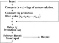  Figure 2.3-10  A flowchart for predictive deconvolution using a prediction filter.

• 

  Figure 2.3-11  A flowchart for predictive deconvolution using a prediction error filter.

• 

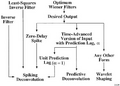  Figure 2.3-12  A flowchart for interrelations between various deconvolution filters.

See also

• Spiking deconvolution
• Prewhitening
• Wavelet processing by shaping filters

External links

find literature about Predictive deconvolution