Synthetic sonic logs

Seismic Data Analysis

Series	Investigations in Geophysics
Author	Öz Yilmaz
DOI	http://dx.doi.org/10.1190/1.9781560801580
ISBN	ISBN 978-1-56080-094-1
Store	SEG Online Store

From the discussion on the convolutional model of a seismic trace in the convolutional model, recall that the starting point was the sonic log (Figure 2.1-8a). The reflection coefficient is defined as the ratio of the reflection amplitude to the incident wave amplitude. In terms of acoustic impedance I = ρα, where ρ is rock density and α is the P-wave velocity, the reflection coefficient c is given by equation (9).

From equation (9), the reflection coefficient is interpreted as the ratio of the change in acoustic impedance to twice the average acoustic impedance. If we assume that density is constant, then equation (9) takes the form

$ c={\frac {A_{1}}{A_{0}}}={\frac {\rho _{2}\alpha _{2}-\rho _{1}\alpha _{1}}{\rho _{2}\alpha _{2}+\rho _{1}\alpha _{1}}}. $

(9)

$ c_{i}={\frac {\alpha _{i+1}-\alpha _{i}}{\alpha _{i+1}+\alpha _{i}}}, $

(56)

where i is the sampling index. Therefore, reflection coefficients can be computed by differentiating the sonic log. The inverse process of getting the interval velocities for synthetic sonic logs from the reflection coefficients, which are assumed proportional to the stacked trace amplitudes, involves integration. In practice, only the high-frequency component of the interval velocity function can be obtained from this inversion. The low-frequency trend must be obtained from other sources of information such as conventional velocity analysis or nearby sonic logs. In many practical situations, there is insufficient well control and the bands of the low- and high-frequency information derived from the seismic data do not overlap. In these cases, problems arise in merging the various types of information; hence, the fidelity of the synthetic sonic logs is degraded.

Lindseth first introduced the concept of synthetic sonic logs and used it in the interpretation of stratigraphic prospects. Figure 11.3-1 illustrates a stacked section with a bright-spot prospect. The corresponding synthetic sonic log section is shown in Figure 11.3-2 wherein the seismic data are superimposed as wiggle traces.

• 
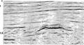  Figure 11.3-1  A portion of a CMP stack containing a bright spot
• 
  Figure 11.3-2  A synthetic sonic log section derived from the stacked section in Figure 11.3-1.

Measured sonic logs generally contain much higher frequencies than seismic data. Integration of seismic traces to get synthetic sonic logs implies a further lowering of the frequency content. A synthetic sonic log and a measured log can only be compared when a high-cut filter is applied to the measured log to make the two appear to have equivalent bandwidths.

The inversion described here is based on the recursive relation in equation (56). Specifically, given values for c_i and α_i, α_i+1 can be computed. Model-based, iterative inversion schemes also exist . These begin with an initial impedance function (specified at a CMP location) from which a synthetic seismogram is computed. This seismogram is crosscorrelated with the actual stack trace at that CMP location. The initial impedance model then is perturbed until the best match is attained between the estimated and actual seismic traces. Finally, inversion techniques, which are based on a certain type of characterization of the reflection coefficient series estimated from stacked data, also exist. For example, the estimated reflection coefficient series can be characterized by a sparse spike series. The sparseness requirement can be satisfied by the condition that the sum of the absolute values of the estimated reflection coefficients is minimum .

Note that regardless of the method, any inversion process suffers from the uncertainty (nonuniqueness) associated with the frequency components outside the dominant seismic signal bandwidth. Thus, the results of the inversion may be questionable for the low-and high-frequency ends of the spectrum at which noise dominates the signal. Constraints (information other than the seismic data being inverted, such as geologic or well control) often are incorporated into inversion schemes used to handle the low-and high-frequency ends of the spectrum.

See also

• Acoustic impedance estimation
• Processing sequence for acoustic impedance estimation
• Derivation of acoustic impedance attribute
• 3-D acoustic impedance estimation
• Instantaneous attributes

External links

find literature about Synthetic sonic logs

References

- ↑ Lindseth (1979), Lindseth, R., 1979, Synthetic sonic logs — a process for stratigraphic interpretation: Geophysics, 44, 3–26.
- ↑ Cooke and Schneider, 1983, Cooke, D. A. and Schneider, W. A., 1983, Generalized linear inversion of reflection seismic data: Geophysics, 48, 665–676.
- ↑ Oldenburg et al., 1983, Oldenburg, D. W., Scheuer, T., and Levy, S., 1983, Recovery of the acoustic impedance from reflection seismograms: Geophysics, 48, 1318–1337.