3-D acoustic impedance estimation
 | |
| Series | Investigations in Geophysics |
|---|---|
| Author | Öz Yilmaz |
| DOI | http://dx.doi.org/10.1190/1.9781560801580 |
| ISBN | ISBN 978-1-56080-094-1 |
| Store | SEG Online Store |
As for the AVO attributes, when derived from 3-D seismic data, an acoustic impedance attribute volume can be used to infer lithology or porosity within a reservoir zone. We shall analyze a land 3-D data set for acoustic impedance estimation. Data specifications for the 3-D seismic data are listed in Table 11-5. The fold of coverage over the survey area is fairly uniform (Figure 11.3-18). In addition to the seismic data, sonic and density logs from a well from within the survey area were used in estimating and removing the constant and linear phase associated with the residual wavelet in the time-migrated CMP stacked data prior to amplitude inversion.
Note the high level of ground-roll energy on the selected shot records with the display gain shown in Figure 11.3-19. The noise characteristics vary from shot to shot. The processing sequence included the following steps:
- Apply t2-scaling to compensate for geometric spreading. Figure 11.3-20a shows a raw shot record and Figure 11.3-20b shows the same record after the application of t2-scaling.
- Perform spiking deconvolution (Figure 11.3-21a).
- Note from the spectral estimate shown in Figure 11.3-22 that deconvolution alone does not flatten the spectrum. Apply time-variant spectral whitening (Figure 11.3-21b) to attain a flat spectrum within the signal passband (Figure 11.3-22d) and attenuate the ground-roll energy.
- Sort the data into common-cell gathers and perform velocity analysis at coarse grid spacing.
- Create a 3-D stacking velocity field and apply NMO correction to the cell gathers.
- Apply residual statics corrections (processing of 3-D seismic data) and inverse NMO correction using the velocity field from step (e).
- Perform velocity analysis at tight grid spacing and create a new 3-D velocity field.
- Apply NMO correction to the cell gathers from step (f), mute and stack.
- Perform poststack deconvolution and a wide band-pass filter.
- Apply f − x deconvolution (linear uncorrelated noise attenuation) to attenuate random noise uncorrelated from trace to trace.
- Finally, perform 3-D poststack phase-shift migration. Note from Figure 11.3-23 that the processing sequence described above yields the spectral shape of the data that we wish to input to poststack amplitude inversion — a broadband spectrum with nearly a flat passband.
-
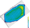 Figure 11.3-18 Fold of coverage map of the land 3-D survey data used in the acoustic impedance case study presented in acoustic impedance estimation.
 -
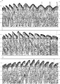 Figure 11.3-19 Part 1: Selected shot records from the 3-D survey data associated with the case study presented in acoustic impedance estimation. (Data courtesy Talisman Energy.)
 -
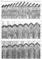 Figure 11.3-19 Part 2: Selected shot records from the 3-D survey data associated with the case study presented in acoustic impedance estimation. (Data courtesy Talisman Energy.)
 -
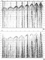 Figure 11.3-20 (a) A raw shot record from the 3-D seismic data associated with the case study presented in acoustic impedance estimation, (b) after geometric spreading correction. (Data courtesy Talisman Energy.)
 -
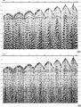 Figure 11.3-21 (a) The same shot record as in Figure 11.3-20b after deconvolution, and (b) time-variant spectral whitening. (Data courtesy Talisman Energy.)
 -
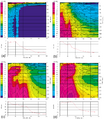 Figure 11.3-22 Amplitude spectrum of the shot record in (a) Figure 11.3-20a, (b) Figure 11.3-20b, (c) Figure 11.3-21a, and (d) Figure 11.3-21b.
 -
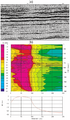 Figure 11.3-23 (a) An inline section from the image volume derived from 3-D poststack time migration, (b) amplitude spectrum of (a).
 -
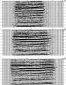 Figure 11.3-24 Part 1: Selected inline sections from the image volume derived from 3-D poststack time migration.
 -
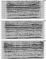 Figure 11.3-24 Part 2: Selected inline sections from the image volume derived from 3-D poststack time migration.
 -
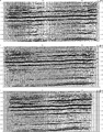 Figure 11.3-24 Part 3: Selected inline sections from the image volume derived from 3-D poststack time migration.
 -
Figure 11.3-24 Part 4: Selected inline sections from the image volume derived from 3-D poststack time migration.


| Survey size | 27.3 km2 |
| Inline dimension | 7.35 km |
| Crossline dimension | 3.75 km |
| Receiver line spacing | 60 m |
| Bin size | 30 × 30 m |
| Number of inlines | 124 |
| Number of crosslines | 245 |
| Number of bins | 30,380 |
| Fold of coverage | 16 |
| Sampling interval | 2 ms |
Figure 11.3-24 shows selected inlines from the image volume derived from 3-D poststack time migration. Following the principle of parsimony in processing for AVO analysis and acoustic impedance estimation, no DMO correction was deemed necessary in the present case study since the subsurface geology can be described by a horizontally layered earth model with no significant faulting or structural distortions.
The next phase in the analysis involves the estimation and removal of the residual phase contained in the time-migrated volume of data. Figure 11.3-25 shows a sonic and a density log measured at a well located at the intersection of inline 76 and crossline 79. Compute the acoustic impedance and the reflectivity series; then, use a zero-phase wavelet with a passband comparable to the signal bandwidth of the seismic data to compute the zero-offset, vertical-incidence synthetic seismogram also shown in Figure 11.3-25. Note from Figure 11.3-26 that the sonic log inserted into a portion of inline 76 at the well location exhibits a very good match with the time-migrated data within the reservoir level indicated by the arrow. To achieve this match, a constant time shift, which is equivalent to a linear phase shift, was applied to the sonic log. A similarly good match is observed in Figure 11.3-27 between the synthetic seismogram and the time-migrated data. To achieve this match, in addition to the constant time shift, a -90-degree phase rotation was applied to the synthetic seismogram. To remove the residual phase in the migrated data set and match it to the zero-phase synthetic seismogram, you therefore need to apply a 90-degree phase rotation to the former.
Figure 11.3-28a shows inline 76 of the image volume from 3-D poststack time migration, and Figure 11.3-28b shows the same section after the 90-degree phase rotation. The phase-rotated image volume is then used in amplitude inversion to create a sparse-spike reflectivity volume. Figure 11.3-28c shows inline 76 from the sparse-spike reflectivity volume. Finally, each sparse-spike reflectivity trace is integrated to estimate the acoustic impedance attribute (Figure 11.3-28d). Selected inlines from the acoustic impedance volume are shown in Figure 11.3-29. These inline traverses coincide with those shown in Figure 11.3-24 from the image volume derived from 3-D poststack time migration before the application of phase rotation.
-
Figure 11.3-25 Log data measured at well location Inline 76 - Crossline 79: (a) the sonic log, (b) the density log, (c) acoustic impedance, (d) the reflectivity series computed from (c) and used in creating (e), and (e) synthetic seismogram using a band-limited wavelet.
-
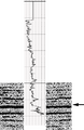 Figure 11.3-26 A portion of Inline 76 from the image volume derived from 3-D poststack time migration with the sonic log as in Figure 11.3-25a inserted at well location, Crossline 79.
 -
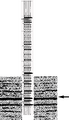 Figure 11.3-27 A portion of Inline 76 as in Figure 11.3-26 from the image volume derived from 3-D poststack time migration with the synthetic seismogram as in Figure 11.3-25e inserted at well location, Crossline 79.
 -
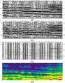 Figure 11.3-28 Cross-sections along inline 76 from (a) the image volume derived from 3-D poststack time migration, (b) the image volume after 90-degree phase rotation, (c) the sparse-spike reflectivity volume, and (d) the acoustic impedance volume.
 -
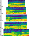 Figure 11.3-29 Part 1: Selected inline sections from the acoustic impedance volume.
 -
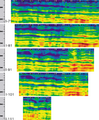 Figure 11.3-29 Part 2: Selected inline sections from the acoustic impedance volume.
 -
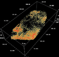 Figure 11.3-30 A 3-D view of the detrital sand level at approximately 850 ms from within the image volume derived from 3-D poststack time migration as in Figure 11.3-24. Red represents high amplitudes.
 -
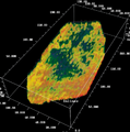 Figure 11.3-31 A 3-D view of the detrital sand level at approximately 850 ms from within the acoustic impedance volume derived from sparse-spike inversion as in Figure 11.3-29. Red represents high impedance values.


The acoustic impedance volume is then interpreted to identify the spatial distribution of high-impedance and low-impedance areas at the reservoir level. First, pick the time horizon at the reservoir level from the image volume and isolate a horizon-consistent thin slab of subvolume. Then, apply transparency to the subvolume to obtain the interpretation result shown in Figure 11.3-30. The red represents the areas of high-amplitude reflections at the reservoir level. Apply the same interpretation strategy to the acoustic impedance volume and obtain a consistent result as shown in Figure 11.3-31. The orange tones represent the zones of high acoustic impedance contrast.
See also
- Acoustic impedance estimation
- Synthetic sonic logs
- Processing sequence for acoustic impedance estimation
- Derivation of acoustic impedance attribute
- Instantaneous attributes
External links
| find literature about 3-D acoustic impedance estimation |