Derivation of acoustic impedance attribute

Seismic Data Analysis

Series	Investigations in Geophysics
Author	Öz Yilmaz
DOI	http://dx.doi.org/10.1190/1.9781560801580
ISBN	ISBN 978-1-56080-094-1
Store	SEG Online Store

As input to poststack amplitude inversion, you may use one of the following data types:

1. A time-migrated CMP-stacked section or volume of data,
2. A CRP-stacked section or volume of data derived from prestack time migration,
3. The intercept AVO attribute section or volume of data (equation 24), or
4. The P-wave reflectivity section or volume of data (equation 37) derived from prestack amplitude inversion.

$R(\theta )=R_{P}+G\sin ^{2}\theta ,$

(24)

$R_{i}=a_{i}{\frac {\Delta \alpha }{\alpha }}+b_{i}{\frac {\Delta \beta }{\beta }},$

(37)

Poststack deconvolution and time-variant spectral whitening (Figures 11.3-5b,c) flatten the spectrum within the passband under the minimum-phase assumption. Nevertheless, there may be residual phase remaining in the stacked data; this residual phase typically is considered to have a constant and a linear phase component. Use of well data makes it possible to estimate the residual phase. After the completion of the conventional processing phase, the residual wavelet in the data input to amplitude inversion needs to be estimated and removed. This requires computing synthetic seismograms at well locations and comparing them with the stacked traces to determine constant-phase and linear-phase components associated with the residual phase left in the migrated data input to amplitude inversion.

1. To start with, inspect and edit available sonic and density logs, and use check-shot information for depth-to-time conversion of the sonic logs (Figure 11.3-8a).
2. Compute the acoustic impedance curve and obtain synthetic seismograms (Figure 11.3-9a) using zero-phase wavelets with a range of bandwidths that cover the passband of the time-migrated stacked data.
3. Apply a range of constant phase rotations (Figure 11.3-9b) to the traces from the time-migrated CMP stacked section at the vicinity of the well and compare the results with the synthetic seismograms. In the present case study, we observed that the time-migrated stack did not require any phase correction within the upper portion of the zone of interest (2.5-3.5 s). Nevertheless, a better match was observed between the well data and the surface seismic data with a constant phase rotation of −90 degrees within the lower portion of the zone of interest (3.5-4.5 s). Figures 11.3-10 and 11.3-11 show portions of the time-migrated stacked section as in Figure 11.3-7 with the application of a constant phase rotation of −90 degrees.
4. Compute a sparse-spike reflectivity model of the earth by a constrained L₁-norm minimization applied to the time-migrated sections in Figures 11.3-10b and 11.3-11b.
5. Apply a mild (3-trace) Karhunen-Loeve filter to the reflectivity sections to remove any spurious, geologically implausable variations in the reflectivity model (Figures 11.3-12a and 11.3-13a).
6. Construct the acoustic impedance model from the broad-band sparse-spike reflectivity model by integrating the reflectivity series at each CMP location (Figures 11.3-12b and 11.3-13b) within the zone of interest (2.5 — 4.5 s).
7. Repeat steps (d), (e), and (f) for the phase-rotated sections in Figures 11.3-10c and 11.3-11c. Results are shown in Figures 11.3-14 and 11.3-15.

• 

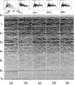  Figure 11.3-5  A portion of the time-migrated CMP stack after: (a) f − x deconvolution, (b) spiking deconvolution, (c) time-variant spectral whitening, (d) time-variant filtering, and (e) Karhunen-Loeve filtering. On top of each panel is the amplitude spectrum averaged over the shot record, and at the bottom is the autocorrelogram.

• 

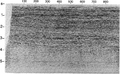  Figure 11.3-7  Migrated CMP stack with poststack processing as in Figure 11.3-5.

• 

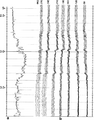  Figure 11.3-8  (a) A portion of the sonic log that spans the time window of interest at one well location on the line shown in Figure 11.3-7 after check-shot correction and depth-to-time conversion; (b) acoustic impedance curves derived from the log in (a), assuming that density is constant, with a range of constant phase rotations.

• 

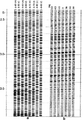  Figure 11.3-9  (a) Synthetic seismograms derived from the impedance curve in Figure 11.3-8 and using a range of pass-bands, with normal (n) and reverse (r) polarity displays; (b) traces from the migrated CMP stacked section in Figure 11.3-7 in the neighborhood of the well location with the sonic log shown in Figure 11.3-8a with a range of constant phase rotations.

• 

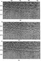  Figure 11.3-10  First portion of: (a) unmigrated CMP stack as in Figure 11.3-6; (b) migrated CMP stack as in Figure 11.3-7; (c) migrated CMP stack with a constant phase rotation of -90 degrees. A display gain has been applied to all three sections.

• 

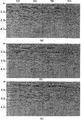  Figure 11.3-11  Second portion of: (a) unmigrated CMP stack as in Figure 11.3-6; (b) migrated CMP stack as in Figure 11.3-7; (c) migrated CMP stack with a constant phase rotation of -90 degrees. A display gain has been applied to all three sections.

• 

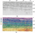  Figure 11.3-12  (a) Broad-band sparse-spike reflectivity section derived from the wide-band time-migrated section shown in Figure 11.3-10b; (b) acoustic impedance section derived from (a).

• 

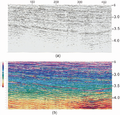  Figure 11.3-13  (a) Broad-band sparse-spike reflectivity section derived from the wide-band time-migrated section shown in Figure 11.3-11b; (b) acoustic impedance section derived from (a).

• 

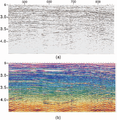  Figure 11.3-14  (a) Broad-band sparse-spike reflectivity section derived from the wide-band time-migrated section shown in Figure 11.3-10c; (b) acoustic impedance section derived from (a).

We applied a range of constant phase rotations to a group of traces at two different locations on the migrated CMP stack and computed the acoustic impedance panels shown in Figures 11.3-16 and 11.3-17. Comparing these panels with the actual impedance curve at the well location (Figure 11.3-8b), we observed that the match between the two impedances in the upper portion of the zone of interest (2.5-3.5 s) is satisfactory without phase rotation applied to the data, while a better match is attained with a 90-degree phase rotation in the lower portion of the zone of interest (3.5-4.5 s). Any discrepancies may be attributed primarily to inaccuracies in the check-shot survey information.

It is important to evaluate the results of amplitude inversion with a cautious perspective. Specifically, one cannot and should not infer individual reservoir properties — pore pressure, confining pressure, porosity, permeability, and fluid saturation, from amplitude inversion. One can only hope to infer a composite effect associated with these properties. Given additional borehole information, however, one may be able to infer that a high impedance value may correspond to, for example, low porosity. In brief, results of amplitude inversion should be used as auxiliary information in support of other tools used in exploration and development of hydrocarbons.

• 

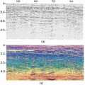  Figure 11.3-15  (a) Broad-band sparse-spike reflectivity section derived from the wide-band time-migrated section shown in Figure 11.3-11c; (b) acoustic impedance section derived from (a).

• 

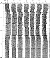  Figure 11.3-16  Part 1: Portion of the acoustic impedance section in Figure 11.3-12b around CMP 370 with constant phase rotations applied.

• 

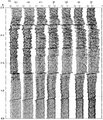  Figure 11.3-16  Part 2: Portion of the acoustic impedance section in Figure 11.3-13b around CMP 370 with constant phase rotations applied.

• 

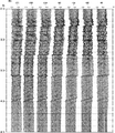  Figure 11.3-17  Part 1: Portion of the acoustic impedance section in Figure 11.3-12b around CMP 450 with constant phase rotations applied.

• 

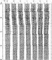  Figure 11.3-17  Part 2: Portion of the acoustic impedance section in Figure 11.3-13b around CMP 450 with constant phase rotations applied.

See also

• Acoustic impedance estimation
• Synthetic sonic logs
• Processing sequence for acoustic impedance estimation
• 3-D acoustic impedance estimation
• Instantaneous attributes

External links

find literature about Derivation of acoustic impedance attribute