Processing of 3-D seismic data
 | |
| Series | Investigations in Geophysics |
|---|---|
| Author | Öz Yilmaz |
| DOI | http://dx.doi.org/10.1190/1.9781560801580 |
| ISBN | ISBN 978-1-56080-094-1 |
| Store | SEG Online Store |
Almost all concepts of 2-D seismic data processing apply to 3-D data processing. Additional complications do arise in 3-D geometry quality control, statics, velocity analysis, and migration. Editing traces with high-level noise, geometric spreading correction, deconvolution and trace balancing, field statics applications (for land and shallow-water data) are done as for 2-D surveys. In conventional 2-D processing, traces are collected into common-midoint (CMP) gathers, while in 3-D processing, traces are collected into common-cell gathers. A common-cell gather coincides with a CMP gather for swath shooting when the lines are straight. Sorting into common-cell gathers introduces special problems. For a dipping reflector, there is the problem of azimuthal variations of the normal moveout (NMO) within the cell for most land data and for marine data with significant cable feathering. While in this section, important aspects of marine and land 3-D processing are discussed, 3-D poststack migration is devoted to 3-D migration.
Figure 7.2-1 is the base map for a land 3-D survey that covers a surface area of nearly 270 km2. The bin size is 25 × 25 m, and there are 520 inlines and 820 crosslines. The 3-D survey presented here comprises more than five million recorded traces, and more than 400,000 stacked traces. Table 7-1 provides a list of the survey parameters.
| Shot interval in m | 25 |
| Group interval in m | 50 |
| Receiver line spacing in m | 500 |
| Number of receiver lines per swath | 6 |
| Number of groups per receiver line | 80 |
| Bin size in m × m | 25 × 25 |
| Fold of coverage | 12 |
| Number of bins per km2 | 1600 |
| Number of bins in the survey | 426,400 |
| Sampling interval in ms | 4 |
| Maximum time in ms | 4000 |
| Number of prestack traces | 5,116,800 |
| Data volume in gigabytes | 20.5 |
Note the irregularities in vibroseis source-array locations — this is mainly a result of cultural restrictions, such as the presence of farm houses and croplands. Figure 7.2-1 also shows a sketch of the recording geometry. There are 6 receiver lines at 500-m intervals, each comprising 80 groups at 50-m intervals. Shots are placed perpendicular to the swath and at the centers of the receiver lines.
Figure 7.2-2 shows selected shot records from the 3-D survey of Figure 7.2-1. Each shot record comprises subrecords each of which corresponds to one of the six receiver lines in the swath. Depending on the shot location relative to the receiver lines in the swath, arrival times of refraction and reflection events vary from one subrecord to another. In some records, ground-roll energy is present; nevertheless, shot records contain generally contain fairly coherent reflection events.
Figure 7.2-3 shows the source and receiver elevations, and the full-fold of coverage over the survey area. Elevations generally increase from southwest to north-east. Note the irregular pattern of the source-array locations and the more-or-less regular layout of the receiver lines in the east-west direction. The average fold of coverage is 12 over the survey area. Note however the variations in fold that follow a regular pattern of striations, and the low-fold area in the center.
-
 Figure 7.2-1 Base map of a land 3-D survey. East is to the right. Shot locations follow the irregular patterns and receiver locations follow the more-or-less regular lines in the east-west direction. Sketch on the bottom right is the recording geometry. See text for details.
 -
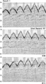 Figure 7.2-2 Part 1: Selected shot records from the 3-D survey of Figure 7.2-1. Note that each shot record comprises subrecords associated with each of the six receivers lines in the swath as sketched in Figure 7.2-1.
 -
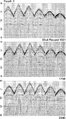 Figure 7.2-2 Part 2: Selected shot records from the 3-D survey of Figure 7.2-1. Note that each shot record comprises subrecords associated with each of the six receivers lines in the swath as sketched in Figure 7.2-1.
 -
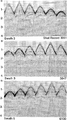 Figure 7.2-2 Part 3: Selected shot records from the 3-D survey of Figure 7.2-1. Note that each shot record comprises subrecords associated with each of the six receivers lines in the swath as sketched in Figure 7.2-1.
 -
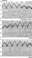 Figure 7.2-2 Part 4: Selected shot records from the 3-D survey of Figure 7.2-1. Note that each shot record comprises subrecords associated with each of the six receivers lines in the swath as sketched in Figure 7.2-1.
 -
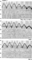 Figure 7.2-2 Part 5: Selected shot records from the 3-D survey of Figure 7.2-1. Note that each shot record comprises subrecords associated with each of the six receivers lines in the swath as sketched in Figure 7.2-1.
 -
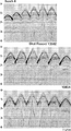 Figure 7.2-2 Part 6: Selected shot records from the 3-D survey of Figure 7.2-1. Note that each shot record comprises subrecords associated with each of the six receivers lines in the swath as sketched in Figure 7.2-1.
 -
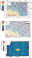 Figure 7.2-3 Top: Source elevations; middle: receiver elevations; bottom: full-fold coverage in the survey area. See the base map in Figure 7.2-1 and the details in the text.
 -
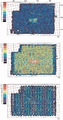 Figure 7.2-4 Fold of coverage maps for near offsets (top), mid-offsets (middle) and far offsets (bottom). See the base map in Figure 7.2-1, full-fold coverage map in Figure 7.2-3, and the details in the text.
 -
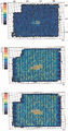 Figure 7.2-5 Fold of coverage maps for source-receiver azimuths that fall within the azimuthal ranges in degrees measured from the north: (340-40) and (160-220) (top); (40-100) and (220-280) (middle); and (280-340) and (100-160) (bottom). See the base map in Figure 7.2-1, full-fold coverage map in Figure 7.2-3, partial-fold coverage maps in Figure 7.2-4, and the details in the text.


Aside from the full-fold coverage map (Figure 7.2-3), it is necessary to examine the fold of coverage for a range of offsets. Figure 7.2-4 shows three coverage maps for offset ranges 0-1000, 1000-2000, and 2000-4000 m. The near-offset fold of coverage appears to be fairly uniform over the survey area. The mid-offset fold of coverage appears to be low and exhibits some variations. Finally, the far-offset fold of coverage map shows that there are bins with missing far-offset traces. Coverage maps are essential to quality control in processing and interpretation. Variations in fold of coverage obviously have undesirable effects on velocity estimation, multiple attenuation, noise attenuation and amplitude variation with offset (AVO) analysis. With missing far offsets, for instance, success in multiple attenuation is compromised.
Fold of coverage should also be examined within the context of source-receiver azimuthal variations. Figure 7.2-5 shows coverage maps for source-receiver azimuths that fall within three ranges — range 1: (340-40) and (160-220); range 2: (40-100) and (220-280); and range 3: (280-340) and (100-160) degrees measured from the north. As a direct consequence of the recording geometry (Figure 7.2-1), the near offsets are largely confined to azimuths that fall in range 1, the middle offsets are largely confined to azimuths that fall in range 2, and the far offsets are largely confined to azimuths that fall in range 3.
See also
- 3-D refraction statics corrections
- Azimuth dependence of moveout velocities
- 3-D dip-moveout correction
- Inversion to zero offset
- Aspects of 3-D DMO correction — a summary
- Velocity analysis
- 3-D residual statics corrections
- 3-D migration
- Trace interpolation
External links
| find literature about Processing of 3-D seismic data |

|

|

|

|

|

|

|