Depth step size

Seismic Data Analysis

Series	Investigations in Geophysics
Author	Öz Yilmaz
DOI	http://dx.doi.org/10.1190/1.9781560801580
ISBN	ISBN 978-1-56080-094-1
Store	SEG Online Store

Finite-difference migration in practice

Finite-difference migration involves downward continuation of the wavefield at the surface, such as a stacked section, and invoking the imaging principle so as to create an image of the subsurface at t = 0. The downward continuation takes place in the computer at discrete depth intervals (migration principles). Depth step size governs performance of finite-difference migration. Inappropriate specification of this parameter can cause artifacts in the migrated section. We want to choose an optimum depth step size that is large for computational savings, yet yields a tolerable error in positioning the events after migration.

Figure 4.3-4 shows the constant-velocity diffraction hyperbola and the 15-degree implicit finite-difference migrations using four different depth steps. Large depth steps cause severe undermigration as well as kinks along the flank of the diffraction curve (especially apparent in the 60- and 80-ms cases). At smaller depth steps, such as the 20- and 40-ms cases, more energy collapses to the apex, but the 15-degree scheme fails to achieve a complete focusing of the energy at the apex of the hyperbola. Note also the dispersive noise that trails the unfocused energy. The dip-limited nature of the 15-degree algorithm, however, causes undermigration whatever the depth step size (Figure 4.3-5).

• 

  Figure 4.3-2  (a) CMP stack, (b) desired migration by phase-shift method, (c) 15-degree finite-difference migration. The finite-difference migration based on the parabolic equation has the inherent property of undermigrating the steep flank of the diffraction and the steeply dipping event. See Figure 4.3-3 for a sketch of the migration results.

• 

  Figure 4.3-3  A sketch of the diffraction D and steeply dipping event before (B) and after (A) desired migration from the sections in Figure 4.3-2. The diffraction and the dipping event after finite-difference migration using the parabolic equation are denoted by FD − D and FD − B, respectively.

• 

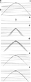  Figure 4.3-4  Tests for extrapolation depth step size in 15-degree finite-difference migration: (a) a zero-offset section that contains a diffraction hyperbola with 2500-m/s velocity, (b) desired migration; 15-degree finite-difference migration using (c) 20-ms (d) 40-ms, (e) 60-ms, and (f) 80-ms depth step.

• 

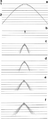  Figure 4.3-5  Tests for extrapolation depth step size in 15-degree finite-difference migration: (a) a zero-offset section that contains a diffraction hyperbola with 2500-m/s velocity, (b) desired migration; 15-degree finite-difference migration using (c) 4-ms (d) 8-ms, (e) 12-ms, and (f) 16-ms depth step.

Undermigration of the diffraction energy along the steep flanks of the hyperbola is caused by the parabolic approximation to the scalar wave equation. The dispersive noise that accompanies the undermigrated energy is an effect of approximating differential operators with difference operators. The accuracy of this approximation decreases at large frequencies and wavenumbers . Thus, the dispersive noise becomes less with smaller trace spacing and sampling in depth and time. For example, the difference operator of equation (10) becomes an increasingly better approximation to the differential operator of equation (11) as Δt is made smaller. To emphasize more strongly the presence of the dispersive noise, migrated sections in Figures 4.3-4 and 4.3-5 have been displayed with the same display gain level as the input section. The dispersion normally is much less pronounced on field data.

${\frac {P(t+\Delta t)-P(t)}{\Delta t}}=a\,P(t).$

(10)

${\frac {dP}{dt}}=a\,P(t).$

(11)

Figure 4.3-6 shows the dipping events model and the 15-degree implicit finite-difference migration results using four different depth step sizes. We can make the following inferences:

1. Increasing depth step size causes more and more undermigration at increasingly steep dips.
2. The waveform along reflectors is dispersed at steep dips and large depth steps.
3. Kinks occur along reflectors at discrete intervals that correspond to the depth step size. Kinks are more pronounced at increasingly steeper dips.

The first inference results from the parabolic approximation, the second from differencing approximations, and the third from gradual undermigration toward the base of each depth step. The kinks are good for diagnostics; their presence indicates that the depth step size that is used is too coarse for the dips present in the data. In that case, smaller depth step size should be used; then the kinks disappear altogether (Figure 4.3-7). Nevertheless, kinks that characterize undermigration can be eliminated by a local adjustment of migration velocities or interpolation between the wavefields at the adjacent depth steps.

It is apparent from Figure 4.3-6 that migration with 20-ms depth step, which corresponds to one-half of the typical dominant period of recorded seismic waves, has the least dispersion with the least undermigration — optimum accuracy in event positioning. Further decreasing depth step size does not improve migration significantly (Figure 4.3-7). The 15-degree implicit scheme causes precursive dispersion at large depth steps greater than 20 ms (Figure 4.3-6) and postcursive dispersion at small depth steps less than 20 ms (Figure 4.3-7). Hence, taking smaller depth steps does not necessarily mean a better quality migration free of the artifacts that occur with the finite-difference method.

Figures 4.3-8 and 4.3-9 show the migrations of the stacked section in Figure 4.3-2a with five different depth steps using the 15-degree implicit scheme. Note that as the depth step size is increased, the dipping event off the flank of the salt diapir is more undermigrated and the diffraction off the tip of the diapir is less collapsed. Dispersion along the diffraction hyperbola is apparent at larger depth steps (Figure 4.3-9). Again, this phenomenon is caused by the differencing approximations to the differential operators used in the design of a finite-difference algorithm.

• 

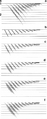  Figure 4.3-6  Tests for extrapolation depth step size in 15-degree finite-difference migration: (a) a zero-offset section that contains dipping events with 3500-m/s velocity, (b) desired migration; 15-degree finite-difference migration using (c) 20-ms (d) 40-ms, (e) 60-ms, and (f) 80-ms depth step.

• 

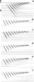  Figure 4.3-7  Tests for extrapolation depth step size in 15-degree finite-difference migration: (a) a zero-offset section that contains dipping events with 3500-m/s velocity, (b) desired migration; 15-degree finite-difference migration using (c) 4-ms (d) 8-ms, (e) 12-ms, and (f) 16-ms depth step.

• 

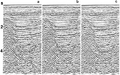  Figure 4.3-8  Tests for extrapolation depth step size in 15-degree finite-difference migration: (a) Desired migration using the phase-shift method, (b) 4-ms depth step, and (c) 20-ms depth step. The input CMP stack is shown in Figure 4.3-2a.

• 

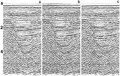  Figure 4.3-9  Tests for extrapolation depth step size in 15-degree finite-difference migration: (a) 40-ms depth step, (b) 60-ms depth step, and (c) 80-ms depth step. The input CMP stack is shown in Figure 4.3-2a and the desired migration is shown in Figure 4.3-2b.

Frequency-space migration in practice

Figure 4.4-6 shows the constant-velocity diffraction hyperbola and the steep-dip implicit 65-degree finite-difference migrations using four different depth steps. Large depth steps cause undermigration as well as kinks along the flank of the diffraction curve (especially apparent in 60- and 80-ms cases). The dispersive noise, typical of finite-difference schemes, persists to varying degrees irrespective of the depth step size. At smaller depth steps, more energy collapses to the apex (Figure 4.4-7f).

As in the case of the parabolic approximation (Figure 4.3-5), the dispersive noise that accompanies the undermigrated energy (Figures 4.4-6 and 4.4-7) is an effect of approximating differential operators with difference operators. With reasonable depth steps (20 ms), the undermigration caused by the dip limitation of the 65-degree algorithm (Figure 4.4-7f) is less pronounced as compared to that of the 15-degree algorithm (Figure 4.3-4c). At large depth steps, the steep-dip accuracy is compromised, and the difference between the two algorithms becomes less distinguishable (compare Figures 4.4-6f and 4.3-4f).

• 

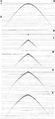  Figure 4.4-6  Tests for extrapolation depth step size in 65-degree frequency-space implicit finite-difference migration: (a) a zero-offset section that contains a diffraction hyperbola with 2500-m/s velocity, (b) desired migration; 65-degree finite-difference migrations using (c) 32-ms, (d) 40-ms, (e) 60-ms, and (f) 80-ms depth step.

• 

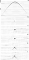  Figure 4.4-7  Tests for extrapolation depth step size in 65-degree frequency-space implicit finite-difference migration: (a) a zero-offset section that contains a diffraction hyperbola with 2500-m/s velocity, (b) desired migration; 65-degree finite-difference migrations using (c) 8-ms, (d) 12-ms, (e) 16-ms, and (f) 20-ms depth step.

The response of a finite-difference algorithm to a diffraction or a dipping event depends upon the type of differencing scheme and dip limitation. At large depth steps, the steep-dip algorithm undermigrates the diffraction hyperbola (Figure 4.4-6) as does the 15-degree scheme (Figure 4.3-4). At small depth steps, the steep-dip algorithm causes slight overmigration of the diffraction hyperbola (Figure 4.4-7c,d), unlike the 15-degree scheme which causes undermigration whatever the depth step size (Figure 4.3-5).

Figure 4.4-8 shows the constant-velocity dipping events model and the steep-dip implicit finite-difference migration results using four different depth step sizes. The response of the steep-dip implicit scheme is quite similar to that of the 15-degree scheme. Specifically, increasing depth step size causes more and more undermigration at increasingly steep dips. The waveform along reflectors is dispersed at steep dips and large depth steps. Kinks occur along reflectors at discrete intervals that correspond to the depth step size. Note that the kinks are more pronounced at increasingly steeper dips.

It is apparent from Figure 4.4-9 that migration with 20-ms depth step has the least dispersion with the least undermigration — optimum accuracy in event positioning. Further decreasing depth step size actually causes overmigration as for the diffraction hyperbola (Figure 4.4-7).

The response of a finite-difference algorithm to dipping events depends again on the approximation made to the scalar wave equation. For instance, with small depth steps less than one-half the dominant period of the reflection events, the steep-dip implicit scheme causes overmigration of the reflection with the steepest dip (Figure 4.4-9c). The 15-degreee implicit scheme, on the other hand, causes postcursive dispersion along the steeply dipping reflectors (Figure 4.3-7c). Hence, taking smaller depth steps does not necessarily mean a better quality migration free of the artifacts that occur with the finite-difference method. With large depth steps, both schemes cause undermigration accompanied by precursive dispersion along the dipping events (Figures 4.3-6 and 4.4-8).

Theoretically, the 65-degree differential equation is more accurate than the 15-degree differential equation. However, once discretized, the difference in performance between these two equations can be less . A good finite-difference migration program uses differencing schemes that maintain the dip accuracy implied by the corresponding differential equation.

The main point to remember is that migration of steep dips generally requires a small depth step size. Practical considerations suggest that depth step size should be between one-half and one-full dominant period of the seismic data to be migrated (from 20 to 40 ms), depending on the steepness of the dips in the data.

A higher order approximation, such as the 65-degree equation, provides a smaller range of choice for optimum depth size as compared to the 15-degree equation. In particular, note that the optimum depth step size is 20 ms for the dipping events model shown in Figures 4.4-8 and 4.4-9; any departure from this value causes either undermigration or overmigration. The results with the 20-ms depth step in Figures 4.3-4 and 4.4-9 convincingly show that the 65-degree algorithm can migrate steeper dips and collapse diffractions more accurately than the 15-degree equation.

Figures 4.4-10 and 4.4-11 show migrations of the stacked section in Figure 4.2-15a with eight different depth steps using a steep-dip implicit scheme. Note that as the depth step size is increased, more undermigration occurs. Dispersion along the undermigrated event associated with the steep left flank of the salt dome is apparent at larger depth steps. A 20-ms depth step size, which is equivalent to the usual case of one-half the dominant period of seismic data, generally is an acceptable choice for most of the implicit finite-difference schemes.

• 

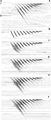  Figure 4.4-8  Tests for extrapolation depth step size in 65-degree frequency-space implicit finite-difference migration: (a) a zero-offset section that contains dipping events with 3500-m/s velocity, (b) desired migration; 65-degree finite-difference migrations using (c) 32-ms, (d) 40-ms, (e) 60-ms, and (f) 80-ms depth step.

• 

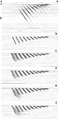  Figure 4.4-9  Tests for extrapolation depth step size in 65-degree frequency-space implicit finite-difference migration: (a) a zero-offset section that contains dipping events with 3500-m/s velocity, (b) desired migration; 65-degree finite-difference migrations using (c) 8-ms, (d) 12-ms, (e) 16-ms, and (f) 20-ms depth step.

• 

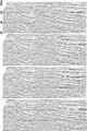  Figure 4.4-10  Tests for extrapolation depth step size in 65-degree frequency-space implicit finite-difference migration using, from top to bottom, 32-ms, 40-ms, 60-ms, and 80-ms depth steps. The input CMP stack is shown in Figure 4.2-15a, and the desired migration using the phase-shift method is shown in Figure 4.2-15b.

• 

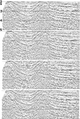  Figure 4.4-11  Tests for extrapolation depth step size in 65-degree frequency-space implicit finite-difference migration using, from top to bottom, 8-ms, 12-ms, 16-ms, and 20-ms depth steps. The input CMP stack is shown in Figure 4.2-15a, and the desired migration using the phase-shift method is shown in Figure 4.2-15b.

Frequency-wavenumber migration in practice

Figure 4.5-5 shows a zero-offset section that contains a set of dipping events migrated with the phase-shift method using different depth step sizes. Since the phase-shift method is based on the dispersion relation given by equation (13b) of the exact one-way wave equation, we do not expect undermigration. However, we see discontinuities along the reflectors at intervals equal to the depth step size, which is similar to the finite-difference results (Figure 4.4-8). As with the finite-difference algorithms, the problem occurs along the steeper dips first; therefore, the steep dips require smaller depth steps (Figure 4.5-5).

$k_{z}={\frac {2\omega }{v}}{\sqrt {1-\left({\frac {vk_{x}}{2\omega }}\right)^{2}}},$

(13b)

Because of the band-limited nature of seismic data, very small depth steps are not needed. From Figure 4.5-5, note that migration with a 20-ms depth step produces a section without spurious kinks along the reflectors; this is comparable to the desired migration using a depth step equal to the temporal sampling interval.

Depth step size tests on field data are shown in Figure 4.5-6. Unlike the finite-difference results (Figure 4.4-10), the phase-shift migration with different depth step sizes produces equally adequate results in terms of the positioning of events. The only problem with large depth steps is the kinks along the steep dips. In principle, as long as there is no aliasing in the z-direction, the depth step kinks can be eliminated by a local interpolation process. In practice, as for the implicit finite-difference methods, the depth step size used in migration with the phase-shift method typically is taken between the half-and full-dominant period of the wavefield — 20 to 40 ms, depending on steepness of the dips present in the section.

• 

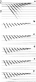  Figure 4.5-5  Tests for extrapolation depth step size in phase-shift migration: (a) a zero-offset section that contains dipping events with 3500-m/s velocity, (b) desired migration; phase-shift migrations using (c) 20-ms (d) 40-ms, (e) 60-ms, and (f) 80-ms depth step.

• 

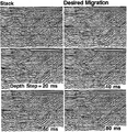  Figure 4.5-6  Tests for extrapolation depth step size in phase-shift migration: Note the kinks along steep dips with large depth steps.

See also

• Velocity errors
• Cascaded migration
• Reverse time migration
• Steep-dip implicit methods
• Steep-dip explicit methods
• Dip limits of extrapolation filters
• Maximum dip to migrate
• Stolt stretch factor
• Wraparound
• Residual migration

External links

find literature about Depth step size

References

- ↑ Claerbout, 1985, Claerbout, J.F., 1985, Imaging the earth’s interior: Blackwell Scientific Publications.
- ↑ Diet and Lailly, 1984, Diet, J.P. and Lailly, P., 1984, Choice of scheme and parameters for optimal finite-difference migration in 2-D: 54th Ann. Internat. Mtg., Soc. Expl. Geophys., Expanded Abstracts, 454–456.