Practical considerations

Seismic Data Analysis

Series	Investigations in Geophysics
Author	Öz Yilmaz
DOI	http://dx.doi.org/10.1190/1.9781560801580
ISBN	ISBN 978-1-56080-094-1
Store	SEG Online Store

Figure 6.4-4 shows the modeled CMP gather before and after t²-stretching. Note that the hyperbolas in Figure 6.4-4a are replaced with parabolas in Figure 6.4-4b. The t²-transformation causes compression on data before 1 s and stretching on data after 1 s. As mentioned earlier, a nice property of the parabolic moveout is that it is invariant along the axis t′ = t² for a specific value of velocity (equation 12). The sampling rate along the t²-axis was set equal to t′/n_t, where n_t is the number of samples along the t-axis. There can be a potential problem of aliasing near t = 0, causing frequency distortion for shallow events. This problem can be avoided by finer sampling along the t′-axis.

By using the singular-value decomposition procedure described in Section F.3, we obtain the Radon transform represented by the velocity-stack gather in the stretched coordinates as shown in Figure 6.4-4c. Finally, we undo the stretching to get the Radon transform represented by the velocity-stack gather in Figure 6.4-4c. Compare this with the conventional velocity-stack gather in Figure 6.4-2d. Note the significant reduction of amplitude smearing and enhancement of velocity resolution in the velocity-stack gather based on the Radon transform. In particular, multiples and primaries now are clearly distinguishable. Nevertheless, there is some frequency distortion of the wavelet associated with the shallowest event in the Radon transform (Figure 6.4-4d), primarily because of stretching and unstretching.

By using the Radon transform (Figure 6.4-5a), the CMP gather can be faithfully reconstructed (Figure 6.4-5b). Compare the panels in Figure 6.4-5 with those in Figure 6.4-3. Note that, unlike the conventional velocity-stack gather, repeated application of the Radon transformation always reproduces the CMP gather with minimal amplitude distortion (Figures 6.4-5b and 6.4-5d), with the exception of frequency distortion at the very early times.

To summarize the construction of velocity-stack gathers using the conventional procedure defined by equation (10a) and the Radon transform based on equation (16), we refer to Figures 6.4-6 and 6.4-7. Starting with the synthetic CMP gather (Figure 6.4-6a), we use equation (10a) to get the conventional velocity-stack gather (Figure 6.4-6b), and the reconstructed gather from it (Figure 6.5-6c) using equation (10b). Again, starting with the same synthetic CMP gather (Figure 6.4-7a), we obtain the velocity-stack gather based on the Radon transform (Figure 6.4-7b) defined by equation (16), and the reconstructed gather from it (Figure 6.4-7c) using equation (10b). It is important to note that the reconstruction procedure using equation (10b) to obtain the modeled CMP gather is the same in both Figures 6.4-6 and 6.4-7. The difference lies in the way the velocity-stack gather is created — the conventional approach causes amplitude smearing along the velocity axis (Figure 6.4-6c), and the procedure based on the Radon transform reduces this smearing and thus increases the resolution along the velocity axis (Figure 6.4-7c).

• 

  Figure 6.4-2  (a) A synthetic CMP gather with three primary reflections; (b) a synthetic CMP gather with one primary reflection (arrival time at 0.2 s at zero-offset time) and its multiples; (c) composite CMP gather containing the primaries and multiples in (a) and (b); (d) the conventional velocity-stack gather derived from the composite CMP gather using equation (10a). Note the amplitude smearing along the velocity axis.

• 

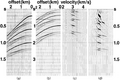  Figure 6.4-4  (a) The CMP gather of Figure 6.4-2c before, and (b) after t²-stretching — note the vertical axis is in units of t²; (c) the velocity-stack gather that represents the Radon transform of (b) using the singular-value decomposition procedure described in Section F.3; (d) the same velocity-stack gather as in (c) after undoing the t²-stretching.

• 

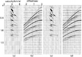  Figure 6.4-5  (a) The same velocity-stack gather as in Figure 6.4-4d; (b) the CMP gather reconstructed from the velocity-stack gather in (a) using equation (10b); (c) velocity-stack gather that represents the Radon transform of (b) using the singular-value decomposition procedure described in Section F.3; (d) CMP gather reconstructed from (c) using equation (10b). Note the accurate reconstruction of the CMP gather (b) from the proper velocity-stack gather (a) compared to the reduction of far-offset amplitudes on the CMP gather in Figure 6.4-3b reconstructed from the conventional velocity-stack gather in Figure 6.4-3a.

• 

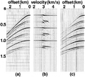  Figure 6.4-6  (a) Synthetic CMP gather; (b) conventional velocity-stack gather; (c) reconstructed CMP gather.

• 

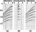  Figure 6.4-7  (a) Synthetic CMP gather; (b) velocity-stack gather based on the discrete Radon transform; (c) reconstructed CMP gather.

• 

  Figure 6.4-8  (a) The synthetic CMP gather as in Figure 6.4-2c; (b) the same gather with added band-limited random noise; (c) the conventional velocity-stack gather (b); (d) the discrete Radon transform of (b). Note the improved velocity resolution in (d) as compared to the amplitude smearing in (c).

• 

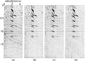  Figure 6.4-9  (a) Velocity-stack gathers associated with the noise-contaminated CMP gather shown in Figure 6.4-8b estimated using β factors incorporated into the computation of the discrete Radon transform based on equation (16): (a) 0.01 percent, (b) 0.5 percent, (c) 1 percent, and (d) 5 percent.

• 

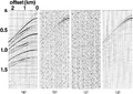  Figure 6.4-10  (a) The modeled CMP gather reconstructed from the velocity-stack gather shown in Figure 6.4-8d; (b) the difference between the modeled CMP gather in (a) and the actual CMP gather in Figure 6.4-8b; (c) the noise component present in the actual CMP gather in (a); (d) difference between (b) and (c). Ideally, (d) should contain zero amplitudes.

Now we examine the performance of the Radon transform in the presence of random noise. Consider the CMP gather in Figure 6.4-8a after the addition of band-limited random noise that is uncorrelated from trace to trace (Figure 6.4-8b). Figure 6.4-8c shows the conventional velocity-stack gather constructed by using equation (10a), and Figure 6.4-8d shows the velocity-stack gather constructed by using the Radon transform based on equation (16). When the data are contaminated by noise, choice of the damping factor β to stabilize the solution represented by equation (16) has a significant impact on the quality of the velocity-stack gather. It is important to emphasize that for the velocity-stack construction using the hyperbolic discrete Radon transform, noise is anything but hyperbolic events.

The β factor is equivalent to the prewhitening factor in Wiener-Levinson deconvolution. In this regard, the optimum β factor depends significantly upon the noise level in the data. Figure 6.4-9 shows estimates of the velocity-stack gathers using four different values of the β factor. For the noise-free case (Figure 6.4-7), theoretically, the best choice of β should be zero; however, to avoid exaggeration of numerical roundoff errors, β should be chosen to be a very small number. A practical rule of thumb is that stability in the SVD procedure does not improve further for β factors beyond a certain value (compare Figures 6.4-9c and d). For field data, a value of 1% of the largest eigenvalue of the matrix L^T*L of equation (16) often yields adequate results (Section F.3).

Since the elements of the matrix L in equation (16) depends on the geometry of the CMP gather under consideration, estimation of the Radon transform u would normally require singular-value decomposition (equation F-22) for each individual gather. To circumvent the repeated application of the singular-value decomposition — a numerically intensive scheme, the Radon transform estimation procedure can be made efficient by implementing a two-staged computation. First, the part of the Radon transform associated with the operator L^T* in equation 16) can be computed using the actual offset distribution of the input CMP gather. Second, the part of the Radon transform associated with the operator (L^T*L)^-1 is computed by the singular-value decomposition only once for the entire data set using an offset distribution that may be considered an acceptable average of the actual offset distributions of the CMP gathers along the line traverse.

Finally, we examine the ability of the Radon transform in separating hyperbolic events from band-limited random noise. Consider the same noisy gather as in Figure 6.4-8b. Reconstruct this CMP gather as shown in Figure 6.4-10a using the velocity-stack gather shown in Figure 6.4-8d, and subtract the result from the original noisy CMP gather (Figure 6.4-8b). This difference gather is shown in Figure 6.4-10b, and it represents the least-squares error e defined as the difference between the actual CMP gather d and the modeled CMP gather d′ defined by equation (15). Ideally, it should contain anything but hyperbolic events. Nevertheless, the missing high-frequency components in the shallowest part of the reconstructed CMP gather have leaked into the difference gather (Figure 6.4-10d). The actual random noise added to the original CMP gather (Figure 6.4-8a) is shown in Figure 6.4-10c. Compare the extracted noise (Figure 6.4-10b) with the actual noise (Figure 6.4-10c) and note that the difference between the two (Figure 6.4-10d) contains negligibly small residual amplitudes aside from some remnants of the hyperbolic events.

Equations

$u(v,\tau )=\sum _{h}d(h,t={\sqrt {\tau ^{2}+4h^{2}\!/\!v^{2}}})$

(10a)

$d'(h,\ t)=\sum _{v}u(v,\tau ={\sqrt {t^{2}-4h^{2}\!/\!v^{2}}})$

(10b)

$t'=\tau '+{\frac {4h^{2}}{v^{2}}}.$

(12)

$\mathbf {d} '=\mathbf {Lu} .$

(15)

$\mathbf {u} =(\mathbf {L^{T\ast }L} )^{-1}\mathbf {L^{T\ast }d} ,$

(16)

See also

• Velocity-stack transformation
• The discrete Radon transform
• The parabolic radon transform
• Impulse response of the velocity-stack operator
• Field data examples
• Radon-transform multiple attenuation

External links

find literature about Practical considerations