Downward continuation

Seismic Data Analysis

Series	Investigations in Geophysics
Author	Öz Yilmaz
DOI	http://dx.doi.org/10.1190/1.9781560801580
ISBN	ISBN 978-1-56080-094-1
Store	SEG Online Store

The harbor experiment described above can be simulated in the computer. Pretend that moving the receiver cable from the beach into the water closer to the barrier is like moving the receiver cable from the surface down into the earth closer to the reflectors. Think of the gap on the barrier as equivalent to a point diffractor on a reflecting interface causing the diffraction hyperbola (Figure 4.1-17a). Start with the wavefield recorded at the surface and move the receivers down to depth levels at finite intervals. Downward continuation of the upcoming wavefield at the surface, therefore, can be considered equivalent to lowering the receivers into the earth.

The computer-simulated wavefields at these different depths are shown in Figure 4.1-17. By applying the imaging principle at each depth, the entire wavefield is imaged. The final output from this process is the migrated section. The last section (panel f) at 1250 m has only one arrival at t = 0. The recording cable is on the storm barrier and the arrival from the gap occurs at t = 0. As the cable moved into the ocean and recorded closer to the barrier, the recorded diffraction hyperbola arrived earlier, and became shorter and more compressed. It collapsed to a point when the receivers coincided with the storm barrier over which the source point forms a gap.

There is one important difference between the physical experiment in Figure 4.1-16 and the computer-simulated downward-continuation experiment in Figure 4.1-17. The receiver cable is the same at each step in Figure 4.1-16, whereas the effective cable length gets shorter and shorter toward the source (the gap in the barrier) in Figure 4.1-17. This is because we started by recording the wavefield at the surface (Figure 4.1-16a) with a finite cable length. The recorded information is confined to within the two raypaths depicted on the section in Figure 4.1-17a. As the cable moves closer to the source, the effective receiver cable containing the information is confined to smaller and smaller lengths. Although receivers are lowered vertically, energy moves down along raypaths it originally took on the way up.

To relate these recordings at different depths (Figure 4.1-17), we superimpose them as shown in Figure 4.1-18a. Moreover, the recordings can be shifted so that the apexes of the hyperbolas coincide and are positioned at a time that is equivalent to the distance from the surface to the diffractor as shown in Figure 4.1-18b. This is called time retardation.

Reconsider the results from the computer simulation of the harbor experiment in Figure 4.1-17. Suppose we stopped recording at a depth of 1000 m before the barrier. The original hyperbola in Figure 4.1-17a was partially collapsed at this depth (Figure 4.1-17e). Therefore, downward continuing to a depth short of the true depth of the source causes undermigration. Diffractions and dipping events also are undermigrated if incorrectly low velocities are used for migration.

• 

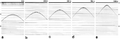  Figure 4.1-16  Moving the receiver cable in the harbor experiment (Figure 4.1-9) from the beach into the water at discrete intervals parallel to the beach line. Numbers on top indicate the distance of the receiver cable from the beach line.

• 

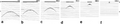  Figure 4.1-17  Computer simulation of the experiment illustrated in Figure 4.1-16. Here, we downward continue the receivers at discrete depth intervals. The numbers on top indicate the distance of the receiver cable from the surface, z = 0.

• 

  Figure 4.1-9  The gap in the barrier acts as Huygens’ secondary source, causing the circular wavefronts that approach the beach line. Adapted from Claerbout .

• 

  Figure 4.1-18  (a) Superposition of the time sections in Figure 4.1-17; (b) removing the translational effect by retardation to place the energy at the apex of the hyperbola obtained initially along the beach line.]]

Assume that the recording continues and passes beyond barrier position z₃ (Figure 4.1-9). We infer that the focused energy on the section at this depth (Figure 4.1-17f) would propagate through the focal point and turn into hyperbolas that are the mirror images of those in Figures 4.1-17a through 4.1-17e. We have downward continued more than necessary. This yields overmigration, which also is caused by incorrectly high velocities. From these observations, note that downward continuing to a wrong depth is like downward continuing with the wrong velocity .

Another important issue to consider is how often the extrapolated wavefield should be computed. When going from one frame to another in Figure 4.1-17, what should the depth step size be? This is discussed in detail later in finite-difference migration in practice.

See also

• Kirchhoff migration
• Diffraction summation
• Amplitude and phase factors
• Kirchhoff summation
• Finite-difference migration
• Differencing schemes
• Rational approximations for implicit schemes
• Reverse time migration
• Frequency-space implicit schemes
• Frequency-space explicit schemes
• Frequency-wavenumber migration
• Phase-shift migration
• Stolt migration
• Summary of domains of migration algorithms

External links

find literature about Downward continuation

References

- ↑ Claerbout, 1985, Claerbout, J.F., 1985, Imaging the earth’s interior: Blackwell Scientific Publications.
- ↑ Doherty and Claerbout, 1974, Doherty, S.M. and Claerbout, J.F., 1974, Velocity analysis based on the wave equation: Stanford Expl. Proj., Rep. No. 1, Stanford University.