Cascaded migration
 | |
| Series | Investigations in Geophysics |
|---|---|
| Author | Öz Yilmaz |
| DOI | http://dx.doi.org/10.1190/1.9781560801580 |
| ISBN | ISBN 978-1-56080-094-1 |
| Store | SEG Online Store |
To compensate for the inherent undermigration by the 15-degree finite-difference migration, Larner and Beasley [1] proposed performing migration using the 15-degree equation, repeatedly — the input to the next migration stage being the output from the previous stage. Such cascaded application of the 15-degree migration is demonstrated in Figure 4.3-17. Migration of the constant-velocity diffraction hyperbola using the 15-degree equation only once yields the familiar result of unfocused energy accompanied with dispersive noise (Figure 4.3-17c). A cascaded application of the 15-degree equation produces improved focusing of the energy at the apex of the hyperbola. The more the number of stages in the cascaded migration the more the improvement in focusing the energy (Figures 4.3-17d,e,f).
An interesting theoretical observation is that cascaded migration using a dip-limited algorithm, such as the 15-degree finite-difference scheme, actually requires a depth step size that is greater than the optimal depth size for a single-stage application of the algorithm. In fact, the more the number of stages in the cascade, the coarser the depth step size to achieve better focusing of the energy (Figure 4.3-17).
-
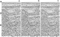 Figure 4.3-8 Tests for extrapolation depth step size in 15-degree finite-difference migration: (a) Desired migration using the phase-shift method, (b) 4-ms depth step, and (c) 20-ms depth step. The input CMP stack is shown in Figure 4.3-2a.
 -
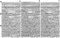 Figure 4.3-9 Tests for extrapolation depth step size in 15-degree finite-difference migration: (a) 40-ms depth step, (b) 60-ms depth step, and (c) 80-ms depth step. The input CMP stack is shown in Figure 4.3-2a and the desired migration is shown in Figure 4.3-2b.
 -
 Figure 4.3-10 Tests for velocity errors in 15-degree finite-difference migration: (a) a zero-offset section that contains a diffraction hyperbola with 2500-m/s velocity, (b) desired migration; 15-degree finite-difference migration using (c) the medium velocity of 2500 m/s, (d) 5 percent lower, (e) 10 percent lower, and (f) 20 percent lower velocity. Depth step size is 20 ms.
 -
 Figure 4.3-11 Tests for velocity errors in 15-degree finite-difference migration: (a) a zero-offset section that contains a diffraction hyperbola with 2500-m/s velocity, (b) desired migration; 15-degree finite-difference migration using (c) the medium velocity of 2500 m/s, (d) 5 percent higher, (e) 10 percent higher, and (f) 20 percent higher velocity. Depth step size is 20 ms.
 -
 Figure 4.3-12 Tests for velocity errors in 15-degree finite-difference migration: (a) a zero-offset section that contains dipping events with 3500-m/s velocity, (b) desired migration; 15-degree finite-difference migration using (c) the medium velocity of 3500 m/s, (d) 5 percent lower, (e) 10 percent lower, and (f) 20 percent lower velocity. Depth step size is 20 ms.
 -
 Figure 4.3-13 Tests for velocity errors in 15-degree finite-difference migration: (a) a zero-offset section that contains dipping events with 3500-m/s velocity, (b) desired migration; 15-degree finite-difference migration using (c) the medium velocity of 3500 m/s, (d) 5 percent higher, (e) 10 percent higher, and (f) 20 percent higher velocity. Depth step size is 20 ms.
 -
 Figure 4.3-14 Tests for velocity errors in 15-degree finite-difference migration using (a) 95 percent, (b) 90 percent, and (c) 80 percent of rms velocities. The input stacked section is shown in Figure 4.3-2a and the desired migration using the phase-shift method is shown in Figure 4.3-2b. Depth step size is 20 ms.
 -
 Figure 4.3-15 Tests for velocity errors in 15-degree finite-difference migration using (a) 105 percent, (b) 110 percent, and (c) 120 percent of rms velocities. The input stacked section is shown in Figure 4.3-2a and the desired migration using the phase-shift method is shown in Figure 4.3-2b. Depth step size is 20 ms.
 -
 Figure 4.3-16 The undermigration and overmigration effects from Figures 4.3-14 and 4.3-15. B = dipping event before and A = dipping event after desired migration, D = diffraction before and D′ = diffraction after 15-degree finite-difference migrations, and L = percent lower velocities, and H = percent higher velocities.


Cascaded migration of the constant-velocity zero-offset section that contains dipping events is shown in Figure 4.3-18. Again, the 15-degree finite-difference migration yields the familiar result of undermigrated steeply dipping events accompanied by the dispersive noise. When applied in a cascaded manner, the algorithm positions the steeply dipping events more accurately. With a sufficient number of cascades (Figure 4.3-18f), the 15-degree algorithm can actually position the events as accurately as a 90-degree algorithm applied only once (Figure 4.3-18b). For comparison, the event with the steepest dip (AB) is labeled on the desired migration (Figure 4.3-18b) and the cascaded migration (Figure 4.3-18f).
Unfortunately, the encouraging results from cascaded migration using the 15-degree algorithm shown in Figures 4.3-17 and 4.3-18 are only attainable for a constant-velocity medium. In case of a medium with vertically varying velocity, the cascaded application of the 15-degree algorithm causes overmigration (Figure 4.3-19). While this observation can be verified by theory, the situation can also be remedied by a cleverly implemented form of cascaded migration with a constant velocity used in each stage [1].
Actually, it turns out that cascaded migration theory dictates constant velocity to be used in each stage. If a variable velocity is used, then a 90-degree algorithm such as the phase-shift method is required in lieu of a dip-limited algorithm for each stage. While the cascaded application of a dip-limited finite-difference algorithm with a variable velocity causes overmigration (Figure 4.3-19c), the cascaded application of the phase-shift algorithm with no dip limit yields an accurate image (Figure 4.3-20e).
Since the advancements made in practical implementation of steep-dip implicit and explicit finite-difference schemes, practical use of cascaded migration, however, has been limited.
References
- ↑ 1.0 1.1 Larner and Beasley, 1990, Larner, K. L. and Beasley, C., 1990, Cascaded migrations: improving the accuracy of finite-difference migration: Geophysics, 52, 618–643.
See also
External links
| find literature about Cascaded migration |