Earth modeling and imaging in depth

Seismic Data Analysis

Series	Investigations in Geophysics
Author	Öz Yilmaz
DOI	http://dx.doi.org/10.1190/1.9781560801580
ISBN	ISBN 978-1-56080-094-1
Store	SEG Online Store

Imaging beneath irregular water bottom in the Northwest Shelf of Australia

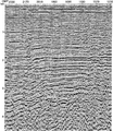
To correct for the effect of the irregular water-bottom topography associated with the reef on the geometry of target reflectors within the substratum, we shall perform earth modeling and imaging in depth. The procedure for earth modeling includes coherency inversion combined with poststack depth migration. Start the analysis by interpreting a set of six time horizons (including the water bottom) within the 0-2.5 s time window from the unmigrated CMP stack (Figure 10.3-1). The time horizons are superimposed on the stacking velocity field in Figure 10.3-2. These time horizons were assumed to be equivalent to zero-offset reflection times and, as such, were used in coherency inversion.

The combination of coherency inversion to estimate the layer velocities and poststack depth migration to delineate the reflector geometries was applied to the six horizons, one layer at a time, starting at the top. Figure 10.3-4 shows the velocity-depth model based on this procedure. Note that the reef has a low-velocity thin cap and a high-velocity interior. The weight of the reef mass may have caused the sagging of the layer boundaries (H2 and H3) associated with the shallow, unconsolidated sediments.

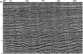
Figure 10.3-5 shows the depth image from prestack depth migration using the velocity-depth model in Figure 10.3-4. Note that the pull-up effect below the reef seen in the time-migrated section (Figure 10.3-3) has been removed. The shelf slope dipping up from left to right is evident from the substratum reflector geometries.

Selected image gathers along the line shown in Figure 10.3-6 contain flat events associated with primaries and events with large moveout associated with multiples. No attempt was made in this case study to attenuate multiples. Conventional CMP stacking attenuates multiples based on velocity discrimination between primaries and multiples. The image gathers in Figure 10.3-6 can be considered similar to CMP gathers that have been moveout corrected using primary velocities. As a result, primaries are flattened and multiples are undercorrected. Therefore, stacking of image gathers to obtain a depth image has a bonus effect of attenuating multiples. However, multiples can make analysis of image gathers for residual moveout a difficult task.

Flatness of the primary events implies the accuracy of the velocity-depth model (Figure 10.3-4) and the accuracy of the depth image (Figure 10.3-5). Compare the depth images derived from prestack depth migration (Figure 10.3-5) and poststack depth migration (Figure 10.3-7) using the same velocity-depth model (Figure 10.3-4). The overmigration effect at the reef edges is quite evident on the poststack depth-migrated section. On the other hand, we remind ourselves the fundamental notion about earth modeling and imaging in depth from introduction to earth modeling in depth — the depth image in Figure 10.3-5 can only be considered a plausable representation of the subsurface geology, and it is not the only representation. Three-dimensional effects increase the ambiguity in the earth model estimated from 2-D seismic data.

• 
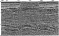  Figure 10.3-1  The Offshore Australia line: unmigrated CMP stack. (Data courtesy Schlumberger Geco-Prakla.)
• 
  Figure 10.3-2  The Offshore Australia line: stacking velocity field with the time horizons interpreted from the unmigrated CMP-stacked section shown in Figure 10.3-1.
• 
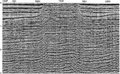  Figure 10.3-3  The Offshore Australia line: poststack time-migrated CMP stack.
• 
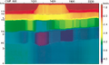  Figure 10.3-4  The Offshore Australia line: velocity-depth model based on layer-by-layer application of coherency inversion and poststack depth migration.
• 
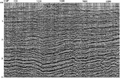  Figure 10.3-5  The Offshore Australia line: depth image from prestack depth migration using the velocity-depth model shown in Figure 10.3-4. Poststack spiking deconvolution, band-pass filtering and AGC scaling were applied.
• 
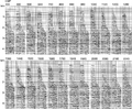  Figure 10.3-6  The Offshore Australia line: selected image gathers associated with the depth image from prestack depth migration shown in Figure 10.3-5.
• 
  Figure 10.3-7  The Offshore Australia line: depth image from poststack depth migration using the velocity-depth model shown in Figure 10.3-4. Compare with the depth image from prestack depth migration shown in Figure 10.3-5.

Imaging beneath volcanics in the West of the Shetlands of the Atlantic Margin

Start the analysis by interpreting a set of six time horizons, including the water bottom and the unconformity itself, within the overburden from the time-migrated CMP stack (Figure 10.4-2). Then, use these time horizons to obtain the unmigrated time horizons by way of a zero-offset traveltime modeling scheme based on image-ray tracing. The modeled time horizons are assumed to be equivalent to zero-offset reflection times, which are then used in coherency inversion. Except for the water bottom, the following sequence is applied to the five horizons, one layer at a time, starting at the top.

1. Perform coherency inversion along the line to estimate the layer velocities, and
2. Perform image-ray depth conversion of the time horizons to delineate the reflector geometries associated with the layer boundaries.
3. Repeat steps (a) and (b) for all five layers within the overburden down to the unconformity and create a velocity-depth model for the overburden (the upper portion of the model that includes the top five layers in Figure 10.4-3b).
4. Assign a range of constant velocities to the half-space that corresponds to the substratum (the region below the unconformity A in Figure 10.4-3b) while using the same overburden model (the region down to the unconformity A in Figure 10.4-3b) and perform prestack depth migration to generate image gathers at some interval along the line.
5. Sort the image gathers into velocity panels as shown in Figures 10.4-4 through 10.4-8.
6. At a specific midpoint location, examine the moveout of events for flatness. Identify the velocity for which there exists a group of flat events within a depth range. The velocity-depth picks are indicated by the left-arrows in Figures 10.4-4 through 10.4-8. Note that for a velocity-depth pick to be valid, not only the event at that depth must be flat but also all events above it must be flat. If we were to pick an rms velocity function at an analysis location as was demonstrated in Figures 5.4-16 through 5.4-19, for the present case, we would only need to create one velocity panel. As an example, the rms velocity picks are denoted by the right-arrows in Figure 10.4-5.
7. Combine the picks for the velocity-depth pairs that meet the flatness criterion at each analysis location and create a layer velocity profile (labeled as VL1 in Figure 10.4-3a) and a layer boundary.
8. Insert the “velocity layer” (labeled as VL1 in Figure 10.4-3b) into the velocity-depth model and define a new half-space region below (Figure 10.4-3b).
9. Then, repeat steps (d) through (h) for the remaining velocity layers — VL2, VL3, and VL4.
10. Perform prestack depth migration (Figure 10.4-9) using the final velocity-depth model shown in Figure 10.4-3b.

Compare the results of from prestack depth migration (Figure 10.4-9) and poststack time migration (Figure 10.4-2), and note that an event (labeled as C) within the substratum has been uncovered. This event is at a depth of 3 km at the left edge of the section and dips down to the right. Also note that the complex structure — which may have a 3-D character — below 4 km between midpoints 440-1240 is imaged within the accuracy of 2-D migration.

Selected image gathers along the line (Figure 10.4-10) largely contain flat events associated with primaries, since multiples were attenuated by way of the Radon transform prior to prestack depth migration. Flatness of the primary events demonstrates the accuracy of the velocity-depth model (Figure 10.4-3) and the accuracy of the depth image (Figure 10.4-9). Note that a spatially varying mute has been applied to image gathers (Figure 10.4-10) to attain an optimum depth image.

Figure 10.4-11 shows depth-to-time conversion of the depth image shown in Figure 10.4-9. The conversion was done using the same velocity field that was used for prestack depth migration (Figure 10.4-3). This section should be compared with the time image derived from poststack time migration shown in Figure 10.4-2. Again, note the event at 3 s (labeled as C) in Figure 10.4-11; this event is almost impossible to follow in Figure 10.4-2.

• 
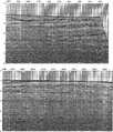  Figure 10.4-2  The West of Shetlands line: poststack time-migrated CMP stack.
• 
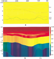  Figure 10.4-3  The West of Shetlands line: (a) layer velocity profiles as functions of midpoint location for the velocity layers — VL1, VL2, VL3, and VL4, within the substratum region below the unconformity labeled as horizon A in the velocity-depth model shown in (b). Above the unconformity, the model was estimated using coherency inversion and image-ray depth conversion; and below the unconformity, the model was estimated using prestack depth migration and moveout analysis of image gathers (as in Figures 10.4-4 through 10.4-8).
• 
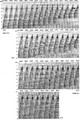  Figure 10.4-4  The West of Shetlands line: prestack depth migration velocity panels at midpoint 241 used in estimating the substratum model (the region below unconformity A in Figure 10.4-3). Shown here are the velocity panels associated with four velocity layers within the substratum — VL1, VL2, VL3, and VL4. The left-arrows ← denote the interval velocity-depth picks and the right-arrows → denote the rms velocity picks. See text for details.
• 
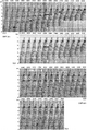  Figure 10.4-5  The West of Shetlands line: prestack depth migration velocity panels at midpoint 321 used in estimating the substratum model (the region below unconformity A in Figure 10.4-3). Shown here are the velocity panels associated with four velocity layers within the substratum — VL1, VL2, VL3, and VL4. The left-arrows ← denote the interval velocity-depth picks. See text for details.
• 
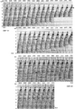  Figure 10.4-6  The West of Shetlands line: prestack depth migration velocity panels at midpoint 401 used in estimating the substratum model (the region below unconformity A in Figure 10.4-3). Shown here are the velocity panels associated with four velocity layers within the substratum — VL1, VL2, VL3, and VL4. The left-arrows ← denote the interval velocity-depth picks. See text for details.
• 
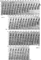  Figure 10.4-7  The West of Shetlands line: prestack depth migration velocity panels at midpoint 721 used in estimating the substratum model (the region below unconformity A in Figure 10.4-3). Shown here are the velocity panels associated with four velocity layers within the substratum — VL1, VL2, VL3, and VL4. The left-arrows ← denote the interval velocity-depth picks. See text for details.
• 
  Figure 10.4-8  The West of Shetlands line: prestack depth migration velocity panels at midpoint 801 used in estimating the substratum model (the region below unconformity A in Figure 10.4-3). Shown here are the velocity panels associated with four velocity layers within the substratum — VL1, VL2, VL3, and VL4. The left-arrows ← denote the interval velocity-depth picks. See text for details.
• 
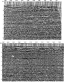  Figure 10.4-9  The West of Shetlands line: depth image from prestack depth migration using the velocity-depth model shown in Figure 10.4-3. Poststack time-variant filtering and AGC scaling were applied. For event C, compare with Figure 10.4-2.
• 
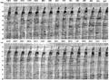  Figure 10.4-10  The West of Shetlands line: selected image gathers associated with the depth image from prestack depth migration shown in Figure 10.4-9.
• 
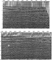  Figure 10.4-11  The West of Shetlands line: depth image from prestack depth migration shown in Figure 10.4-9 converted to time domain using the velocity-depth model shown in Figure 10.4-3. Poststack time-variant filtering and AGC scaling were applied. For event C, compare with Figure 10.4-2.
• 
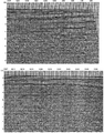  Figure 10.4-12  The West of Shetlands line: depth image from prestack depth migration using the velocity-depth model shown in Figure 10.4-3 and prestack data without Radon-transform multiple attenuation. Poststack time-variant filtering and AGC scaling were applied. Compare with the depth image in Figure 10.4-9 derived from data with Radon-transform multiple attenuation.
• 
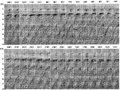  Figure 10.4-13  The West of Shetlands line: selected image gathers associated with the depth image from prestack depth migration shown in Figure 10.4-12. Compare with the image gathers in Figure 10.4-10 derived from data with Radon-transform multiple attenuation.
• 
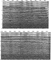  Figure 10.4-14  The West of Shetlands line: depth image from prestack depth migration shown in Figure 10.4-12 converted to time domain using the velocity-depth model shown in Figure 10.4-3. Poststack time-variant filtering and AGC scaling were applied. Compare with the results in Figure 10.4-11.

This case study also included a test of the effect of multiples on prestack depth migration. The image gathers shown in Figure 10.4-10 and the corresponding depth image shown in Figure 10.4-9 are based on prestack data with Radon-transform multiple attenuation. Using the same velocity-depth model (Figure 10.4-3), but prestack data without multiple attenuation, prestack depth migration yields the depth image shown in Figure 10.4-12. Note the overwhelming presence of multiples in this depth image; in contrast, the depth image in Figure 10.4-9 is largely free of multiples.

Now examine the image gathers with and without multiple attenuation (Figures 10.4-10 and 10.4-13). Primary events are flat or nearly flat, whereas events associated with multiples have significant moveout. The multiples dominate the image gathers so much that the moveout analyses shown in Figure 10.4-4 through 10.4-8 could not have been conducted using data without multiple attenuation.

Figure 10.4-14 shows depth-to-time conversion of the depth image shown in Figure 10.4-12. Again, as in Figure 10.4-11, the conversion was done using the same velocity field that was used for prestack depth migration (Figure 10.4-3). Note that the event that is distinctively identified in Figure 10.4-11 (labeled as C) is somewhat contaminated by the strong multiples in Figure 10.4-14.

Imaging beneath shallow gas anomalies in the Gulf of Thailand

To resolve the effect of shallow gas anomalies, we shall perform earth modeling and imaging in depth. The procedure for earth modeling includes coherency inversion to estimate layer velocities combined with image-ray depth conversion to delineate reflector geometries. Start the analysis by interpreting a set of eight time horizons within the 0-2.5 s time window from the time-migrated CMP stack (Figure 10.5-3). These time horizons are used to obtain the unmigrated time horizons by way of ray-theoretical zero-offset modeling. The modeled time horizons are assumed to be equivalent to zero-offset reflection times, which are then used in coherency inversion.

Figure 10.5-4 shows the velocity-depth model based on the procedure outlined above. Note the lateral velocity variations within the layers in the neighborhood of the faulted zones. Figure 10.5-5 shows the depth image from prestack depth migration using the velocity-depth model in Figure 10.5-4. Note the crisp image of the fault below midpoint 2170 and the structural closures along the fault line between 1.5-2.5 km. Another feature of interest is the v-shaped structure centered around midpoint 1370. The boundaries of the closure defined by the two faults that merge at a depth of approximately 2.4 km below midpoint 1370 are not coincident with the changes in the reflector geometries because of faulting. This most likely is caused by the 3-D behavior of the fault, which is not imaged properly by 2-D depth migration.

Selected image gathers along the line shown in Figure 10.5-6 convincingly demonstrate the accuracy of the velocity-depth model (Figure 10.5-4). The flatness of events on the image gathers also provides evidence of the accuracy of the depth image (Figure 10.5-5). Compare the depth images derived from prestack depth migration (Figure 10.5-5) and poststack depth migration (Figure 10.5-7) using the same velocity-depth model (Figure 10.5-4). Although both are better than time migration (Figure 10.5-3), prestack depth migration yields a better image of the faults and the deep, subtle structural closures.

• 
  Figure 10.5-3  The Gulf of Thailand line: poststack time-migrated CMP stack.
• 
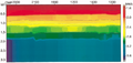  Figure 10.5-4  The Gulf of Thailand line: velocity-depth model based on a layer-by-layer application of coherency inversion and image-ray depth conversion.
• 
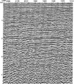  Figure 10.5-5  The Gulf of Thailand line: depth image from prestack depth migration using the velocity-depth model shown in Figure 10.5-4. Poststack deconvolution and AGC scaling were applied.
• 
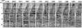  Figure 10.5-6  The Gulf of Thailand line: selected image gathers associated with the depth image from prestack depth migration shown in Figure 10.5-5.
• 
  Figure 10.5-7  The Gulf of Thailand line: depth image from poststack depth migration using the velocity-depth model shown in Figure 10.5-4. Depth image from prestack depth migration is shown in Figure 10.5-5.

This case study demonstrates that seismic inversion for earth modeling and imaging in depth is not required just for targets below obviously complex structures (subsalt imaging in the North Sea and subsalt imaging in the Gulf of Mexico), but can also be required for resolving low-relief structures in the presence of subtle, shallow velocity anomalies.

See also

• Imaging beneath irregular water bottom in the Northwest Shelf of Australia
• Imaging beneath volcanics in the West of the Shetlands of the Atlantic Margin
• Imaging beneath shallow gas anomalies in the Gulf of Thailand

External links

find literature about Earth modeling and imaging in depth