The need for imaging in three dimensions
 | |
| Series | Investigations in Geophysics |
|---|---|
| Author | Öz Yilmaz |
| DOI | http://dx.doi.org/10.1190/1.9781560801580 |
| ISBN | ISBN 978-1-56080-094-1 |
| Store | SEG Online Store |
Figure 7.0-1 shows a CMP-stacked section from an area with very complex subsurface geology. As we examine the subsurface structure inferred by this section starting from the left side, we see a section from top to bottom with good-quality reflections. Then, most likely because of surface conditions, there is a zone of virtually no reflection. The remaining part of the section gives the appearance of very tight anticlinal features cascaded on top of one another. Nevertheless, it is most likely that these features have a strong 3-D aspect. The important point is that even if we were able to supply the correct migration velocity field for the section in Figure 7.0-1, 2-D migration of this 2-D cross-section of a 3-D wavefield would not yield the correct subsurface image.
We have always recorded 3-D seismic wavefields since the beginnings of the seismic method. A 2-D seismic profile is merely a cross-section of a truly 3-D propagating wavefield. Until the mid-1970s, we have been recording cross-sections of 3-D wavefields and processing as if the wavefield is 2-D, rather than 3-D. Although we still continue conducting 2-D seismic surveys for regional exploration, since the mid-1980s, 3-D seismic surveys have been used for prospect generation and detailed delineation of oil and gas reservoirs.
3-D effects can be minimized on 2-D lines by choosing the dominant dip direction as the shooting direction. For instance, in areas with structures that have resulted from overthrust tectonics, 2-D lines are traversed perpendicular to thrust fronts. Nevertheless, you will certainly need strike lines to tie the dip lines.
If there are any 3-D effects on a 2-D line, they can often be recognized. Figure 7.0-2 shows a CMP-stacked section before and after migration. Follow the unconformity A on the migrated section — events appear geologically plausable until we encounter an interfering feature B at the steep flexure. This event is not immediately correlatable with other events on the section, and is almost certainly out-of-plane. Although coherent on its own, it simply does not belong to the plane of this section. Only after 3-D migration of a 3-D volume of stacked data, will this event be imaged at its correct subsurface location. As a result of 3-D migration, this sideswipe event will have moved out of the plane of the section in Figure 7.0-2.
The section shown in Figure 7.0-3 unambiguously demonstrates the need for 3-D migration of 3-D data to achieve a complete and accurate imaging of the subsurface. The stacked section (Figure 7.0-3a) indicates irregular topography associated with a sea-bottom canyon. At first impression, there should be no problem in imaging the water-bottom reflector correctly. All you need to do is Stolt migration using the constant velocity associated with the water layer. The result shown in Figure 7.0-3b exhibits significant undermigration of the event associated with the water bottom. In other words, we have not achieved a complete and accurate imaging even though we used the correct migration velocity.
If it is not an erroneously too-low velocity, then what is the cause of this undermigration? To seek the answer to this question, consider the earth model in Figure 7.0-4, which consists of a dipping plane interface in a homogeneous medium. Examine line A along the dip direction. If the survey consisted of lines parallel to the dip direction, then a 2-D assumption about the subsurface would be valid. No out-of-plane signal would be recorded and 2-D migration of these dip lines would be correct, as shown in Figure 7.0-5a. After 2-D migration, point D beneath surface point X is migrated updip to its true subsurface position D′. Now consider line B, which is in the strike direction in Figure 7.0-4. Line B ties line A at surface position X. The reflection from the subsurface point D′ in Figure 7.0-5a is recorded on both lines A and B at their intersection point X. The event on line B is an out-of-plane reflection, while the event on line A is not. However, the reflection on the strike line from the dipping interface shows no dip (Figure 7.0-5b). Since migration does not alter the position of flat events, the migrated section for the strike line is identical to the corresponding unmigrated section. While the unmigrated sections associated with the dip line A and the strike line B would tie, after migrating both sections, a mistie would occur (Figure 7.0-5b).
-
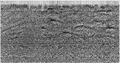 Figure 7.0-3 A 2-D CMP-stacked section (a) before, and (b) after migration.
 -
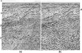 Figure 7.0-2 A 2-D CMP-stacked section (a) before, and (b) after migration.
 -
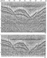 Figure 7.0-3 A 2-D CMP-stacked section (a) before, and (b) after migration.
 -
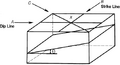 Figure 7.0-5 (a) Migration along the dip line and (b) along the strike line over the depth model in Figure 7.0-4. Point D after migration is moved updip to D′ along dip line A. Point D does not move after migration along strike line B. This causes the mistie indicated between the two migrated sections.
 -
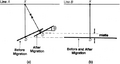 Figure 7.0-5 (a) Migration along the dip line and (b) along the strike line over the depth model in Figure 7.0-4. Point D after migration is moved updip to D′ along dip line A. Point D does not move after migration along strike line B. This causes the mistie indicated between the two migrated sections.


The subsurface generally dips in many directions in areas where structural traps of interest exist. Thus, it is not possible to identify the inline direction as either a dip or strike direction. This is the case for line C in Figure 7.0-4. Examine the positioning after migration of point D beneath intersection point X for all three lines in the plan view in Figure 7.0-6. Point D is moved to the true subsurface position D′ along dip line A. The same point does not move after migration along strike line B. It moves to D″ along line C. Note that the lateral displacement DD″ along the oblique line C is less than the lateral displacement DD′ along the dip line. This is because the apparent dip perceived along the oblique line is less than the true dip of the plane interface that is perceived along the dip line. For accurate positioning, a second pass of migration is suggested in the direction perpendicular to line C to move the already migrated energy from D″ to its true subsurface position D′.
Principles of 3-D migration are discussed in 3-D poststack migration. Here, we shall assess the interpretational differences between 2-D and 3-D migrations. Figure 7.0-7 shows an inline (left column) and a crossline (right column) stacked section from a land 3-D survey. Pretend that these two sections are from a 2-D survey and migrate them individually to get the 2-D migrated sections. Then, take the entire volume of 3-D stacked data and perform 3-D migration, and subsequently display the data corresponding to these lines. Note that 3-D migration has yielded a better definition of the top T of the salt dome and better delineation of the faults along the base B of the salt dome. There is no doubt that the interpretation based on 2-D imaging is significantly different from interpretation based on 3-D imaging. It is not really a question of which section has the most lateral continuity of events — what matters is the accuracy of imaging we achieve from 2-D versus 3-D migration.
Figure 7.0-8 shows another example of the significant improvement available from the interpretation of a 3-D migrated section. Note that the two salt domes and the syncline between are delineated better after 3-D migration. The zone between the two salt domes exhibits undermigrated events on the 2-D migrated section (Figure 7.0-8b) in the same manner as described in Figure 7.0-6.
Three-dimensional migration often produces surprisingly different sections from 2-D migrated sections. The example in Figure 7.0-9 shows a no-reflection zone on the 2-D migrated section, while the same zone contains a series of continuous reflections on the 3-D migrated section that are easily correlated with reflections outside that zone. The 2-D migrated section exhibits the shadow events associated with the sideswipe energy masking the continuous reflections in the middle portion of the section. When we do 2-D migration, we confine the movement of the energy into the plane of the line itself. So the energy contained in the unmigrated stacked section in Figure 7.0-9 is indeed the same as the energy contained in the 2-D migrated section — only that it has been moved somewhere else on the section. As a result of moving the energy during 3-D migration within the 3-D volume, some moved into the plane of the section as in Figure 7.0-9 from others and some moved out of the section and migrated into the others.
-
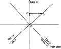 Figure 7.0-6 Plan view of the migrations at the intersection point along the three lines indicated in Figure 7.0-4. Point D moves to D′, its true subsurface position, along dip line A. Point D does not move on strike line B. The same point moves to D″ along line C, which is in an arbitrary direction. Complete imaging is achieved by migrating the data again along the direction perpendicular to C to move the energy from D″ to D′.
 -
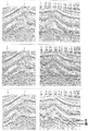 Figure 7.0-7 An inline (top left) and a crossline (top right) stacked section from a land 3-D survey. Also shown are the 2-D (center row) and 3-D (bottom row) migrations of the two stacked sections. (Data courtesy Nederlandse Aardolie Maatschappij B.V.)
 -
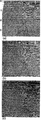 Figure 7.0-8 (a) An inline stacked section from a marine 3-D survey, (b) 2-D migration, (c) 3-D migration. (Data courtesy Amoco Europe and West Africa, Inc.)
 -
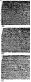 Figure 7.0-9 (a) Another inline stacked section from the same marine 3-D survey as in Figure 7.0-8, (b) 2-D migration, (c) 3-D migration. (Data courtesy Amoco Europe and West Africa, Inc.)


As noted earlier, 2-D migration can introduce misties between 2-D lines in the presence of dipping events. Two-dimensional migration cannot adequately image the subsurface, while 3-D migration eliminates these misties by completing the imaging process. From the field data examples, we see that 3-D migration provides complete imaging of the 3-D subsurface geology. In contrast, 2-D migration can yield inadequate results. The difference between 2-D seismic and 3-D seismic is the way in which migration is performed. Dense coverage on top of a target zone, say a 12.5-m inline trace spacing and a 25-m crossline trace spacing, will not necessarily provide adequate subsurface imaging unless migration is performed in a 3-D sense.
Cable feathering in marine 3-D surveys and swath shooting geometry in land 3-D surveys give rise to source-receiver azimuthal variations. As a direct consequence of this acquisition-related phenomenon, stacking velocities become not only dip dependent but also azimuth dependent. 3-D dip-moveout correction fortunately accounts for both dip and azimuth effects on stacking velocities. Figure 7.0-10 shows an inline section from a 3-D poststack migrated data from a 3-D marine survey with 3-D DMO correction applied. This data set represents a case of events with conflicting dips — specifically, the steeply dipping fault plane reflections and the gently dipping reflections associated with the sedimentary strata. Note that 3-D DMO correction has preserved both of these events. This then enabled 3-D migration to produce a crisp image of the fault planes.
Figure 7.0-11 shows an inline section from a land 3-D survey. Note that the inline stacked section without 3-D DMO correction (Figure 7.0-11a) exhibits poor stacking along the steep flanks of the salt dome, particularly above 1 s. There is no apparent case of conflicting dips in this section along the salt flanks. What causes the poor stacking performance is the large source-receiver azimuthal variations that arise from the swath shooting geometry. After the application of 3-D DMO correction, the reflections along the steep flanks of the salt dome are now preserved on the stacked section (Figure 7.0-11b). Clearly, the quality of 3-D migration hinges upon the quality of the stacked volume of data. Compare the sections in Figures 7.0-11c and 7.0-11d, and note that 3-D migration of the data with 3-D DMO correction yields a better delineation of the salt dome geometry. The improvement resulting from 3-D DMO correction is primarily within the overburden above the salt dome. The subsalt region should not be affected fundamentally by 3-D DMO correction since this region is adversely influenced by the raypath distortions caused by the complex overburden associated with the top-salt boundary. As such, the imaging problem in the subsalt region is not within the realm of 3-D DMO correction and 3-D time migration; instead, it is a problem that needs to be handled by 3-D imaging in depth.
Recall from introduction to migration that different migration strategies are required for different types of subsurface geological circumstances (Table 4-1). Consider the case of conflicting dips with different stacking velocities associated with fault-plane reflections and the surrounding sedimentary strata. The marine data set shown in Figures 7.0-12 through 7.0-17 exhibits such a case. The section shown in Figure 7.0-12a represents the CMP stack along an inline traverse with no DMO correction. As such, fault-plane reflections have not been preserved and the 2-D poststack time migration of this stacked section yields a poor image of the fault planes (Figure 7.0-12b).
| Case | Migration |
| dipping events | time migration |
| conflicting dips with different stacking velocities | prestack migration |
| 3-D behavior of fault planes and salt flanks | 3-D migration |
| strong lateral velocity variations associated with complex overburden structures | depth migration |
| complex nonhyperbolic moveout | prestack migration |
| 3-D structures | 3-D migration |
Since this data set is an inline extracted from a 3-D marine survey, traces in the CMP gathers have source-receiver azimuthal variations that result from cable feathering and multi-cable recording geometry. To correct for the source-receiver azimuthal effect on moveout and therefore stacking velocities, one needs to do 3-D, rather than 2-D, DMO correction (processing of 3-D seismic data). In contrast with the conventional stack (Figure 7.0-12a), note the presence of fault-plane reflections on the 3-D DMO stack shown in Figure 7.0-13a. If, however, the fault planes have a 3-D geometry, then 2-D poststack time migration still falls short of providing a good image of the subsurface (Figure 7.0-13b).
-
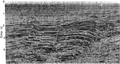 Figure 7.0-10 A cross-section from a 3-D poststack time-migrated volume of 3-D DMO-stacked data.
 -
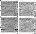 Figure 7.0-11 (a) A cross-section from a 3-D volume of CMP-stacked data associated with a land 3-D survey without 3-D DMO correction; (b) with 3-D DMO correction; (c) same cross-section as in (a) after 3-D poststack time migration; (d) same cross-section as in (b) after 3-D poststack time migration.
 -
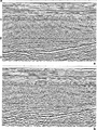 Figure 7.0-12 (a) A CMP-stacked section derived from common-cell gathers along an inline from a 3-D marine survey; (b) 2-D poststack time migration of the CMP-stacked section in (a). (Data courtesy Gulf Canada.)
 -
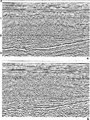 Figure 7.0-13 (a) 3-D DMO stack of the data as in Figure 7.0-12; (b) 2-D poststack time migration of the 3-D DMO stack in (a).


To correct for conflicting dips with different stacking velocities, strictly, one needs to do prestack, and not poststack, time migration (prestack time migration). However, prestack time migration, when performed in 2-D, once again falls short of meeting the accurate imaging requirements (Figure 7.0-14a). Because of the acoustic impedance changes along the fault planes caused by the juxtaposition of velocities across the fault blocks, it is useful to examine the migrated section in Figure 7.0-14a also with its polarity reversed (Figure 7.0-14b).
Imaging in 3-D alone would not provide a good image if the input stacked volume of data does not contain the fault-plane reflections (Figure 7.0-15). By combining 3-D DMO correction and 3-D poststack time migration (Figure 7.0-16), the imaging quality for the fault-plane reflections is greatly enhanced. The ultimate imaging solution in the time domain to the problem of conflicting dips with different stacking velocities is 3-D prestack time migration (Figure 7.0-17).
-
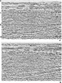 Figure 7.0-14 (a) 2-D prestack time migration of the data as in Figure 7.0-12; (b) the same section as in (a) displayed with reverse polarity.
 -
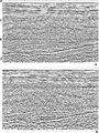 Figure 7.0-15 (a) A CMP-stacked section derived from common-cell gathers along an inline from a 3-D marine survey (the same section as in Figure 7.0-12a); (b) the same inline section as in (a) after 3-D poststack time migration.
 -
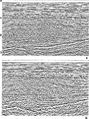 Figure 7.0-16 (a) A DMO-stacked section derived from common-cell gathers along an inline from a 3-D marine survey (the same section as in Figure 7.0-13a); (b) the same inline section as in (a) after 3-D poststack time migration.
 -
 Figure 7.0-17 (a) The same inline section as in Figure 7.0-16 after 3-D prestack time migration; (b) the same section as in (a) displayed with reverse polarity.


See also
- Introduction to 3-D seismic exploration
- 3-D survey design and acquisition
- Processing of 3-D seismic data
- 3-D poststack migration
- 3-D prestack time migration
- Interpretation of 3-D seismic data
- Exercises
- Mathematical foundation of 3-D migration
External links
| find literature about The need for imaging in three dimensions |