Azimuth dependence of moveout velocities

Seismic Data Analysis

Series	Investigations in Geophysics
Author	Öz Yilmaz
DOI	http://dx.doi.org/10.1190/1.9781560801580
ISBN	ISBN 978-1-56080-094-1
Store	SEG Online Store

Following the application of field statics, data are sorted into common-cell gathers. The swath shooting geometry used commonly in land 3-D surveys produces common-cell gathers in which all midpoints coincide with the cell center. However, this technique also can result in large variations in the source-receiver azimuths and, thus, can result in traveltime deviations similar to or greater than those caused by midpoint scattering in marine surveys.

Consider a land 3-D recording geometry that comprises a range of shot-receiver azimuths as in Figure 7.2-5. Much as in the case of cable feathering (Figure 7.1-11), reflections from a dipping interface do not align along a single hyperbolic moveout curve. Instead, source-receiver azimuthal variations give rise to travel time deviations from the ideal hyperbolic moveout. Using a single velocity for the NMO correction would yield a stacked trace with high frequencies attenuated, again as in the case of cable feathering (Figure 7.1-12).

Stack attenuation increases with the increasing shot-receiver azimuth range. If this attenuation is serious, correction for the shot-receiver azimuth before stacking is needed. At first, it appears that this may be achieved by grouping the traces in a CMP gather into various ranges of azimuths and applying different velocities for moveout correction of each group of traces. Nevertheless, as we shall discuss shortly, 3-D DMO process implicitly corrects for the effect of source-receiver azimuth on moveout velocities.

• 

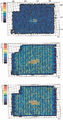  Figure 7.2-5  Fold of coverage maps for source-receiver azimuths that fall within the azimuthal ranges in degrees measured from the north: (340-40) and (160-220) (top); (40-100) and (220-280) (middle); and (280-340) and (100-160) (bottom). See the base map in Figure 7.2-1, full-fold coverage map in Figure 7.2-3, partial-fold coverage maps in Figure 7.2-4, and the details in the text.

• 

  Figure 7.1-11  Traveltimes and the least-squares-fit hyperbolic moveout curves associated with (a) strike-line shooting, (b) shooting in the 45-degree direction from the downdip azimuth, and (c) dip-line shooting. These traveltimes were derived from a single planar interface with a 30-degree dip in a constant-velocity medium. The feathering angle is 10 degrees and midpoint distribution in the cell is shown in Figure 7.1-10. Numbers along the moveout curves denote the lines that contribute midpoints to the cell under study .

• 

  Figure 7.1-12  (a) The stacking operator associated with midpoint scatter along the crossline direction. This operator was derived from traveltime deviations from the best-fit hyperbolic moveout curve in Figure 7.2-3a. (b) The amplitude spectrum suggests that high frequencies are attenuated (causing smearing of stacked amplitudes) because of midpoint scatter .

But first, because of its historical significance, we shall briefly review the azimuth-dependent velocity analysis. Levin in his classic paper developed the equations for moveout velocity and traveltime associated with a dipping reflector and for a source-receiver pair along an arbitrary azimuthal direction measured from the dip line direction. The geometry of Levin’s equations is shown in Figure 7.2-8. In normal moveout, we discussed the normal moveout for the case of a 2-D dipping reflector and derived the respective equations in Section C.3.

The 3-D equivalent of equation (3-10) is

$t^{2}=t_{0}^{2}+{\frac {4h^{2}(1-\sin ^{2}\phi \cos ^{2}\theta )}{v^{2}}},$

(2)

while the 3-D equivalent of equation (3-11) is

$v_{NMO}={\frac {v}{\sqrt {1-\sin ^{2}\phi \cos ^{2}\theta }}},$

(3)

where θ is the azimuth angle between the structural dip direction and the direction of the profile line, ϕ is the dip angle (Figure 7.2-8), t is the two-way traveltime associated with the nonzero-offset raypath from the source location to the reflection point on the dipping interface back to the receiver location, t₀ is the two-way zero-offset time t₀ associated with the normal-incidence ray-path at the midpoint location, v_NMO is the moveout velocity, and v is the velocity of the medium above the dipping reflector.

Figure 7.2-9 shows a plot of the ratio of v_NMO/v based on equation (3) as a function of azimuth angle for a range of dip angles . For a dip line, the azimuth is zero; and for a strike line, the azimuth is 90 degrees. The ratio v_NMO/v is significant when the line is shot at or near the structural dip direction.

Equation (3) describes an ellipse in polar coordinates (Figure 7.2-10). The radial coordinate is the NMO velocity v_NMO, while the polar angle is the azimuth θ. Orientation of the major axis of the velocity ellipse is in the true dip direction.

• 

  Figure 7.2-8  Geometry for a dipping planar interface used in deriving the 3-D moveout equation (2), where ϕ is the dip angle, and θ is the source-receiver azimuth angle measured from the dip line .

• 

  Figure 7.2-9  Graphic representation of the 3-D NMO velocity given by equation (3) and derived from the geometry of Figure 7.2-8, where ϕ is the dip angle and θ is the source-receiver azimuth angle as measured from the dip line. Moveout velocity is identical to medium velocity if the shooting direction is in the strike-line direction (90-degree azimuth). The largest difference between the moveout velocity and the medium velocity occurs along the dip-line direction (zero azimuth) at large dip angles .

• 

  Figure 7.2-10  The 3-D NMO velocity given by equation (3) is an ellipse in polar coordinates. The radial coordinate represents the NMO velocity at a given azimuth, which is the polar angle α. Adapted from .

The velocity ellipse can be constructed based on moveout velocities measured in three different directions. Lehmann and Houba discuss several practical aspects of this measurement. By subgrouping traces from a CMP gather into three different azimuths (α₁, α₂, α₃), the stacking velocities (v_s1, v_s2, v_s3) can be estimated along those azimuths. If the stacking velocities in three different directions are known, then the semi-major and semi-minor axes a and b, respectively, and the orientation (downdip azimuth angle, ε) of the velocity ellipse can be defined (Figure 7.2-10). Once the velocity ellipse is constructed for a dipping reflector at a CMP location, then the following parameters can, in principle, be determined:

1. The true dip of the reflector, ϕ = cos⁻¹(b/a).
2. The downdip azimuth ε.
3. The stacking velocity at any azimuth, $v_{s}=v/{\sqrt {1-\sin ^{2}\phi \cos ^{2}\theta }},$ where v = b (medium velocity above the reflector), and θ is the azimuth angle measured from the major axis a.

This is called the three-parameter velocity analysis. Each trace in the CMP gather is moveout corrected using the velocity along the corresponding shot-receiver azimuth.

A resolution problem arises in practice for the three-parameter velocity analysis. Land 3-D data often are of low fold; so partitioning the data into azimuth ranges with lower folds of coverage may not yield good velocity estimates. Azimuth variations can be minimized on land swath recording by minimizing perpendicular offset of sources from the receivers. Azimuth variation also often is largest on the near offsets where total moveout is small. Thus, the effect of source-receiver azimuth on stacking velocity (equation 2) can be fairly small. Another issue is offset distribution — ideally, it is desirable to have a wide range of offsets for each common-cell gather. Otherwise small errors in moveout correction may cause trace-to-trace chatter on stacked sections. Anyway, we leave the three-parameter velocity analysis and move onto 3-D dip-moveout correction to account for source-receiver azimuth and dip effect on stacking velocities.

See also

• 3-D refraction statics corrections
• 3-D dip-moveout correction
• Inversion to zero offset
• Aspects of 3-D DMO correction — a summary
• Velocity analysis
• 3-D residual statics corrections
• 3-D migration
• Trace interpolation

External links

find literature about Azimuth dependence of moveout velocities

References

- ↑ 1.0 1.1 Bentley and Yang, 1982, Bentley, L. and Yang, M., 1982, Scatter of midpoints grouped in cells and its effects on stacking: unpublished technical document, Western Geophysical Company.
- ↑ 2.0 2.1 2.2 2.3 2.4 Levin (1971), Levin, F. K., 1971, Apparent velocities from dipping interface reflections: Geophysics, 36, 510–516.
- ↑ Lehmann and Houba (1985), Lehmann, H. J. and Houba, W., 1985, Practical aspects of determination of 3-D stacking velocities: Geophys. Prosp., 33, 155–163.