Impulse response of the velocity-stack operator
 | |
| Series | Investigations in Geophysics |
|---|---|
| Author | Öz Yilmaz |
| DOI | http://dx.doi.org/10.1190/1.9781560801580 |
| ISBN | ISBN 978-1-56080-094-1 |
| Store | SEG Online Store |
An isolated spike in the offset domain (Figure 6.4-11a) maps to the velocity domain using equation (10a) along a curved trajectory (Figure 6.4-12a). Solve equation (9b) for v to obtain the equation for this trajectory in the velocity domain:
$ u(v,\tau )=\sum _{h}d(h,t={\sqrt {\tau ^{2}+4h^{2}\!/\!v^{2}}}), $ ()
$ t^{2}=\tau ^{2}+{\frac {4h^{2}}{v^{2}}}, $ ()
$ v={\frac {2h}{\sqrt {t^{2}-\tau ^{2}}}}. $ ()
The curvature is greater for a spike situated at far offset than a spike situated at near offset (Figures 6.4-11b and 6.4-12b). Also, the curvature is greater for a spike situated at an early time on a given offset than a spike situated at a late time on the same offset (Figures 6.4-11c and 6.4-12c).
Inverse transformation of the conventional velocity-stack gathers (Figures 6.4-12a,b,c) back to the offset domain does not reproduce the isolated spikes (Figures 6.4-13a,b,c). Instead, the amplitudes are smeared across each of the CMP gathers. The amplitude smearing is worse for spikes situated at near offsets (Figure 6.4-13b) and late times (Figure 6.4-13c).
Figures 6.4-14a,b,c show the velocity-stack gathers based on the Radon transform of equation (16) associated with the isolated spikes in Figures 6.4-11a,b,c. Inverse mapping these velocity-stack gathers, in contrast with the results obtained from inverse mapping of the conventional velocity-stack gathers (Figures 6.4-13a,b,c), yields a fairly good focusing of energy to the isolated spike locations (Figures 6.4-15a,b,c).
$ \mathbf {u} =(\mathbf {L^{T\ast }L} )^{-1}\mathbf {L^{T\ast }d} , $ ()
How is the velocity-stack processing affected by irregularities in the data? Refer to the CMP gather in Figure 6.4-11d. It contains a trace with a monofrequency signal, another trace with polarity reversed, a dead trace, and another trace with a dead zone. The conventional velocity-stack gather is shown in Figure 6.4-12d, and the CMP gather reconstructed from it is shown in Figure 6.4-13d. Compare this figure with Figure 6.4-11d and note the differences along the reflection hyperbolas in amplitude and curvature where the anomalous traces are located. Also, note the smearing of the monofrequency signal over a large range of traces away from the original trace location. The velocity-stack gather based on the Radon transform associated with the CMP gather in Figure 6.4-11d is shown in Figure 6.4-14d. The CMP gather reconstructed from it (Figure 6.4-15d) shows less smearing of the monofrequency signal. As with the conventional velocity-stack gather, however, the dead trace and the trace with a dead zone in the original CMP gather (Figure 6.4-11d) again have been replaced with nonzero amplitudes, and traveltimes have been distorted along the reflection hyperbolas where the anomalous traces are located.
-
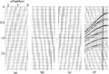 Figure 6.4-11 Synthetic CMP gathers that contain (a) a single spike; (b) a series of spikes at equal time but at different offsets; (c) a series of spikes at equal offset but at different times; (d) anomalous traces.
 -
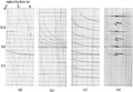 Figure 6.4-12 Conventional velocity-stack gathers associated with the CMP gathers in Figure 6.4-11.
 -
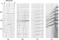 Figure 6.4-13 Reconstructed CMP gathers from the conventional velocity-stack gathers in Figure 6.4-12. Compare with Figure 6.4-11.
 -
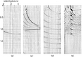 Figure 6.4-14 Velocity-stack gathers that represent the Radon transforms of the CMP gathers in Figure 6.4-11. Compare with Figure 6.4-12.
 -
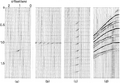 Figure 6.4-15 Reconstructed CMP gathers from the proper velocity-stack gathers in Figure 6.4-14. Compare with Figures 6.4-11 and 6.4-13.


The transform parameters of practical importance are the velocity range and the velocity increment used in constructing velocity-stack gathers. The velocity range should span the velocities associated with primary and multiple reflections. A good practice for the choice of velocity increment is such that the number of traces in velocity space is set equal to the traces in the offset space.
See also
- Velocity-stack transformation
- The discrete Radon transform
- The parabolic Radon transform
- Practical considerations
- Field data examples
- Radon-transform multiple attenuation
External links
| find literature about Impulse response of the velocity-stack operator |