Velocity resolution
 | |
| Series | Investigations in Geophysics |
|---|---|
| Author | Öz Yilmaz |
| DOI | http://dx.doi.org/10.1190/1.9781560801580 |
| ISBN | ISBN 978-1-56080-094-1 |
| Store | SEG Online Store |
Figure 9.2-9 shows the semblance curves derived from coherency inversion at CMP location 75. (Horizon 3 is missing at this location.) The CMP gather itself is shown in Figure 9.2-7a. Note that the sharpness of the peak in the semblance curve, hence the velocity resolution, depends upon the depth of the layer boundary and the magnitude of the layer velocity. Also, recall from Figure 9.1-12 that the velocity resolution also depends on the effective cable length.
The sampling interval for the velocity axis in the semblance curves should be chosen by taking into consideration the velocity resolution that can be achieved. Figure 9.2-10 shows the CMP data windows with the reflections that correspond to the selected horizons. The horizontal axis spans the offset range used in coherency inversion. For shallow horizons (1, 2, and 4), the offset range is smaller because of muting. The CMP gather is shown in Figure 9.2-7a and the semblance curves are shown in Figure 9.2-9. For a given horizon, the data window with the flattest event is distinguishable when the velocity sampling is appropriate. Specifically, for shallow horizons with low velocity (e.g., Horizons 1 and 2), velocity increment needs to be small enough to pick a layer velocity, accurately. However, for deeper events with high velocity (e.g., Horizons 7a and 7e), the velocity increment does not have to be as small, since event curvature in the data windows becomes indistinguishable as seen in Figure 9.2-10. It is only with large velocity increments that we observe a marked difference in event curvature as demonstrated in Figure 9.2-11. A good rule of thumb in practice is that the sampling interval in velocity used in stacking velocity inversion and coherency inversion needs to be specified as small as 25 m/s for velocities as low as 1500 m/s and can be specified as large as 200 m/s for velocities as high as 5000 m/s.
-
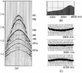 Figure 9.2-7 Coherency inversion for the model in Figure 9.2-1. (a) CMP gather at analysis location CMP 75 as in Figure 9.2-8; (b) semblance curve; (c) data window for three trial velocities. CMP raypaths that correspond to these trial velocities are shown in Figure 9.2-8.
 -
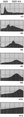 Figure 9.2-9 Semblance curves from coherency inversion at CMP location 75 as in Figure 9.2-8 applied to the horizons as in Figure 9.2-2. The CMP gather is shown in Figure 9.2-7a and the data windows are shown in Figure 9.2-10.
 -
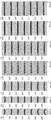 Figure 9.2-10 Data windows from coherency inversion at CMP location 75 as in Figure 9.2-8 applied to the horizons as in Figure 9.2-2. The CMP gather is shown in Figure 9.2-7a and the semblance curves are shown in Figure 9.2-9. True layer velocities are posted at the bottom of each panel.
 -
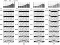 Figure 9.2-11 Data windows and semblance curves from coherency inversion for Horizon 7a at CMP location 75 as in Figure 9.2-8 using velocity increments of (a) 25 m/s, (b) 50 m/s, (c) 100 m/s, and (d) 200 m/s. The CMP gather is shown in Figure 9.2-7a. True layer velocity is 3500 m/s.
 -
 Figure 9.1-12 Semblance spectra derived from coherency inversion applied to the central CMP gather associated with the stacked data in Figure 9.1-1a using maximum offsets of 2400 m, 1400 m, and 400 m. See text for details.


See also
External links
| find literature about Velocity resolution |