Practical aspects of slant stacking

Seismic Data Analysis

Series	Investigations in Geophysics
Author	Öz Yilmaz
DOI	http://dx.doi.org/10.1190/1.9781560801580
ISBN	ISBN 978-1-56080-094-1
Store	SEG Online Store

First, we examine the interrelations between various domains used in seismic data processing. Consider a band-limited dipping event in the t − x domain as shown in Figure 6.3-13. The offset range is from 250 to 5000 m with a trace spacing of 50 m. This event is mapped along a radial line AA′ in the f − k domain.

The slope of the radial line, ω/k_x is related to the horizontal phase velocity v/sin θ by the relationship

$ {\frac {\omega }{k_{x}}}={\frac {v}{\sin \theta }}. $

(6)

• 
  Figure 6.3-13  A single dipping event in various domains.
• 
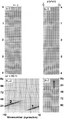  Figure 6.3-14  A spatially aliased single dipping event in various domains.
• 
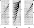  Figure 6.3-15  Slant stacking is invertible: (a) A CMP gather is mapped from t − x domain onto τ − p domain (b), from which the original gather can be reconstructed (c). The linear streaks labeled as CT in (b) are caused by the finite cable length.

Substitute for p = sin θ/v to find the relationship between the variables in the transform domain given by

$ k_{x}=p\omega . $

(7)

Figure 6.3-13 also shows the mapping of the dipping event to the τ − p domain. Note that a linear event in the t − x domain maps onto a point in the τ − p domain. Converse also is true — a linear event in the τ − p domain maps onto a point in the t − x domain.

A 1-D Fourier transform of the slant-stack traces in the time direction gives the amplitude spectrum in the ω − p domain, which also is shown in Figure 6.3-13. Actually, the ω − p plane describes the frequency dependency of horizontal phase velocity and is used in analyzing guided waves (Section F.1). The energy along the radial direction AA′ in the ω − k_x domain is equivalent to that along the vertical direction BB′ in the ω − p domain.

Figure 6.3-14 shows a spatially aliased dipping event. Again, as in Figure 6.3-13, the offset range is from 250 to 5000 m with a trace spacing of 50 m. The wraparound observed in the ω − k_x plane results from the inadequate spatial sampling of the event. Note that both the unaliased component, segment 1, and the aliased component, segment 2, map onto a single p trace. We expect the spatially aliased part to map onto a number of negative p traces. However, if this were the case, then the aliased frequency range (21 to 42 Hz) would be absent from the ω − p plane in which only the positive p values were included.

• 
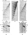  Figure 6.3-16  Slant stack can be used for trace interpolation: (a) a t − x gather is transformed to a τ − p gather (c), and is reconstructed using a finer trace spacing (d). The corresponding f − k spectra show spatial aliasing in the original gather (b), which was eliminated after reconstruction (e).
• 
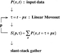  Figure 6.3-8  Construction of slant-stack gathers

We now outline the steps involved in slant-stack processing that includes forward and inverse τ − p transforms.

1. Start with the offset data, apply linear moveout correction for a specified value of p, and sum over offset (equations 4a, 4b). Repeat for a range of p values, the output is the slant-stack gather (Figure 6.3-8).
2. Apply a particular process in the slant-stack domain, such as dip filtering or deconvolution.
3. Apply rho filtering to the processed slant-stack gather.
4. Then, apply inverse linear moveout correction for a specified offset value, and sum over the p-range (equations 5a, 5b). Repeat for all offsets; the output is the slant-stack processed offset data.

$ \tau =t-px, $

(4a)

$ S(p,\tau )=\sum _{x}P(x,\tau +px), $

(4b)

$ t=\tau +px. $

(5a)

$ P(x,t)=\sum _{p}S(p,t-px). $

(5b)

We illustrate the forward and inverse τ − p transforms using the synthetic CMP gather shown in Figure 6.3-15. This figure also shows the slant-stack and reconstructed CMP gather without any process applied, except the rho filter. The linear streaks labeled as CT on the slant-stack gather in Figure 6.3-15 are caused by the finite cable length. To minimize the streaks, for each trace in the t − x domain, Kelamis and Mitchell limit the mapping from the t − x domain to the τ − p domain to a time-variant zone in the τ − p domain. Specifically, only one trace at a time from the t − x domain is mapped onto all p traces. The resulting τ − p gather is muted on both the low and high end of the p-axis in a time-varying manner. The mute functions are based on a representative primary velocity function.

During reconstruction of the t − x gather, we do not have to use the same trace spacing that was used for the original t − x gather. Consider the synthetic CMP gather in Figure 6.3-16a. The 2-D amplitude spectrum shows that frequencies above 48 Hz are spatially aliased (Figure 6.3-16b). This gather can be mapped to the slant-stack domain (Figure 6.3-16c) and reconstructed using a finer trace spacing (Figure 6.3-16d). The original trace spacing is 25 m; the reconstructed gather has a trace spacing of 12.5 m. The 2-D amplitude spectrum of the trace-interpolated gather shows that no frequencies are spatially aliased (Figure 6.3-16e). Nevertheless, note the missing high-frequency energy beyond 60 Hz. This energy mainly is along the steep direct arrival path in the input gather (Figure 6.3-16a) and is absent in the output gather (Figure 6.3-16d). We see that reconstruction can be successful even for spatially aliased data, provided dips do not have a wide range of variation.

See also

• Physical aspects of slant stacking
• Slant-stack transformation
• Slant-stack parameters
• Time-variant dip filtering
• Slant-stack multiple attenuation

External links

find literature about Practical aspects of slant stacking

References

- ↑ Kelamis and Mitchell (1989), Kelamis, P. G. and Mitchell, A. R., 1989, Slant-stack processing: First Break, 7, 43–54.