Wavelet processing by shaping filters

Spiking deconvolution had trouble compressing wavelet (-  1/2, 1) to a zero-lag spike (1, 0, 0) (Table 2-14). In terms of energy distribution, this input wavelet is more similar to a delayed spike, such as (0, 1, 0), than it is to a zero-lag spike, (1, 0, 0). Therefore, a filter that converts wavelet (-  1/2, 1) to a delayed spike would yield less error than the filter that shapes it to a zero-lag spike (Table 2-14).

Figure 2.3-1  A flowchart for Wiener filter design and application.

Table 2-13. Design and application of a two-term least-squares inverse filter (a, b).

Filter Design
Convolution of the filter (a, b) with input wavelet $(-{\frac {1}{2}},\ 1)$:
	-  1/2	1		Actual Output	Desired Output
b	a			−a/2	0
	b	a		−b/2 + a	1
		b	a	b	0
Filter Application
Least-Squares Filter				(0.76, −0.09)
Input Wavelet				(−0.5, 1)
Actual Output				(−0.38, 0.81, −0.09)
Desired Output				(0, 1, 0)

Table 2-14. Error in least-squares filtering.

Input Wavelet: $(-{\frac {1}{2}},\ 1)$
Desired Output	Actual Output	Error Energy
(1, 0, 0)	(0.24, −0.38, 0.19)	0.762
(0, 1, 0)	(−0.38, 0.81, −0.09)	0.190

Recast the filter design and application outlined in Table 2-13 in terms of optimum Wiener filters by following the flowchart in Figure 2.3-1. First, compute the crosscorrelation (Table 2-21). From Table 2-19, we know the autocorrelation of the input wavelet. By substituting the results from Tables 2-19 and 2-21 into the matrix equation (30), we get

Table 2-19. Autocorrelation lags of input wavelet (-  1/2, 1).

	-  1/2	1		Output
	-  1/2	1		5/4
		-  1/2	1	-  1/2

Table 2-20. Crosscorrelation lags of desired output (1, 0, 0) with input wavelet (-  1/2, 1).

	1	0	0	Output
	-  1/2	1		-  1/2
		-  1/2	1	0

Table 2-21. Crosscorrelation lags of desired output (0, 1, 0) with input wavelet (-  1/2, 1).

	0	1	0	Output
	-  1/2	1		1
		-  1/2	1	-  1/2

${\begin{pmatrix}r_{0}&r_{1}&r_{2}&\cdots &r_{n-1}\\r_{1}&r_{0}&r_{1}&\cdots &r_{n-2}\\r_{2}&r_{1}&r_{0}&\cdots &r_{n-3}\\\vdots &\vdots &\vdots &\ddots &\vdots \\r_{n-1}&r_{n-2}&r_{n-3}&\cdots &r_{0}\end{pmatrix}}{\begin{pmatrix}a_{0}\\a_{1}\\a_{2}\\\vdots \\a_{n-1}\\\end{pmatrix}}={\begin{pmatrix}g_{0}\\g_{1}\\g_{2}\\\vdots \\g_{n-1}\end{pmatrix}}$

(30)

${\begin{pmatrix}5/4&-1/2\\-1/2&5/4\\\end{pmatrix}}{\begin{pmatrix}a\\b\\\end{pmatrix}}={\begin{pmatrix}1\\-1/2\end{pmatrix}}.$

(33)

By solving for the filter coefficients, we obtain $\left(a,\ b\right):\left({\frac {16}{21}},\ -{\frac {2}{21}}\right).$ This filter is applied to the input wavelet as shown in Table 2-22. As we would expect, the output is the same as that of the least-squares filter (Table 2-13). Note that, from Table 2-14, the energy of the least-squares error between the actual and desired outputs was 0.190 and 0.762 for a delayed spike and a zero-lag spike desired output, respectively. This shows that there is less error when converting wavelet (-  1/2, 1) to the delayed spike (0, 1, 0) than to zero-lag spike (1, 0, 0).

In general, for any given input wavelet, a series of desired outputs can be defined as delayed spikes. The least-squares errors then can be plotted as a function of delay. The delay (lag) that corresponds to the least error is chosen to define the desired delayed spike output. The actual output from the Wiener filter using this optimum delayed spike should be the most compact possible result.

Table 2-22. Convolution of input wavelet $(-{\frac {1}{2}},\ 1)$ with filter coefficients $\left({\frac {16}{21}},\ -{\frac {2}{21}}\right).$

		-  1/2	1		Output
	-  2/21	-  16/21			−0.38
		-  2/21	-  16/21		0.81
			-  2/21	-  16/21	−0.09

The process that has a type 5 desired output (any desired arbitrary shape) is called wavelet shaping. The filter that does this is called a Wiener shaping filter. In fact, type 2 (delayed spike) and type 4 (zero-phase wavelet) desired outputs are special cases of the more general wavelet shaping.

Figure 2.3-5 shows a series of wavelet shapings that use delayed spikes as desired outputs. The input is a mixed-phase wavelet. Filter length was held constant in all eight cases. Note that the zero-delay spike case (spiking deconvolution) does not always yield the best result (Figure 2.3-5a). A delay in the neighborhood of 60 ms (Figure 2.3-5e) seems to yield an output that is closest to being a perfect spike. Typically, the process is not very sensitive to the amount of delay once it is close to the optimum delay. If the input wavelet were minimum-phase, then the optimum delay of the desired output spike generally is zero. On the other hand, if the input wavelet were mixed-phase, as illustrated in Figure 2.3-5, then the optimum delay is nonzero. Finally, if the input wavelet were maximum-phase, then the optimum delay is the length of that wavelet .

Can we not delay the desired spike output (Figure 2.3-5) and obtain a better result than we obtained from spiking deconvolution? This goal is achieved by applying a constant-time shift (60 ms in Figure 2.3-5) to a delayed spike result. Better yet, the same result can be obtained by shifting the shaping filter operator as much as the delay in the spike and applying it to the input wavelet. Such a filter operator is two-sided (non-causal), since it has coefficients for negative and positive time values. The one-sided filter defined along the positive time axis has an anticipation component, while the filter defined along the negative time axis has a memory component . The two-sided filter has an anticipation component and a memory component. Figure 2.3-6 shows a series of shaping filterings with two-sided Wiener filters for various spike delay values.

• 

  Figure 2.3-4  (a) Minimum-phase wavelet, (b) after band-pass filtering, (c) followed by deconvolution. The amplitude spectrum of the band-pass filtered wavelet is zero above 108 Hz (middle row); therefore, the inverse filter derived from it yields unstable results (bottom row). The time delays on the wavelets in the left frames of the middle and bottom rows are for display purposes only.

• 

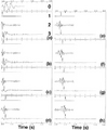  Figure 2.3-5  Shaping filtering. (0) Input wavelet, (1) desired output, (2) shaping filter operator, (3) actual output. Here, the purpose is to convert the mixed-phased wavelet (0) to a series of delayed spikes as shown in (a) through (h) by using a one-sided operator (anticipation component only). The best result is with a 60-ms delay (e).

• 

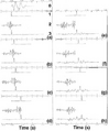  Figure 2.3-6  Shaping filtering. (0) Input wavelet, (1) desired output, (2) shaping filter operator, (3) actual output. Here, the purpose is to convert the mixed-phase wavelet (0) to a series of delayed spikes as shown in (a) through (h) using a two-sided operator (with memory and anticipation components). The best result is obtained with a zero-delay spike using a two-sided filter (a).

Figure 2.3-7 shows examples of wavelet shaping. The input wavelet represented by trace (b) is the same mixed-phase wavelet as in Figure 2.3-6 (top left frame). This wavelet is shaped into zero-phase wavelets with three different bandwidths represented by traces (c), (d) and (e). This process commonly is referred to as dephasing. Figure 2.3-7 shows another wavelet shaping in which the input wavelet is converted to its minimum-phase equivalent represented by trace (f). This conversion is often applied to recorded air-gun signatures.

Figure 2.3-8 shows examples of a recorded air-gun signature that was shaped into its minimum-phase equivalent and into a spike. When the input is the recorded signature, then the wavelet shapings in Figure 2.3-8 are called signature processing.

Wavelet shaping requires knowledge of the input wavelet to compute the crosscorrelation column on the right side of equation (30). If it is unknown, which is the case in reality, then the minimum-phase equivalent of the input wavelet can be estimated statistically from the data. This minimum-phase estimate then is shaped to a zero-phase wavelet.

Wavelet processing is a term that is used with flexibility. The most common meaning refers to estimating (somehow) the basic wavelet embedded in the seismogram, designing a shaping filter to convert the estimated wavelet to a desired form, usually a broad-band zero-phase wavelet (Figure 2.3-8), and finally, applying the shaping filter to the seismogram. Another type of wavelet processing involves wavelet shaping in which the desired output is the zero-phase wavelet with the same amplitude spectrum as that of the input wavelet (Figure 2.3-9). Note that this type of wavelet processing does not try to flatten the spectrum, but only tries to correct for the phase of the input wavelet, which sometimes is assumed to be minimum-phase.

• 

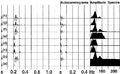  Figure 2.3-7  Shaping filtering with various desired outputs. (a) Impulse response, (b) input seismogram. Here, (c), (d) and (e) show three possible desired outputs that are band-limited zero-phase wavelets, while (f) shows a desired output that is the minimum-phase equivalent of the input wavelet (b). Finally, (g) and (h) are desired outputs that are band-pass filtered versions of (f).

• 

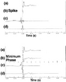  Figure 2.3-8  Signature processing: (a) Recorded signature, (b) desired output, (c) shaping operator, (d) shaped signature. The desired output is a zero-delay spike (top) and the minimum-phase equivalent of the recorded signature (bottom).

• 

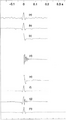  Figure 2.3-9  Wavelet processing. An autocorrelogram (a), estimated from the seismic trace, is used after smoothing (b) to compute the spiking deconvolution operator (d). Here (c) is just a one-sided version of (b). The inverse of the operator (d) is the minimum-phase wavelet (e), which is sometimes assumed to be the basic wavelet contained in the original seismic trace. It is easy to compute its zero-phase equivalent (f) and design a shaping filter (g) that converts the minimum-phase wavelet (e) to the zero-phase wavelet (f). The actual output is (h), which should be compared with (f). The zero-phase equivalent (f) has the same amplitude spectrum as the minimum-phase wavelet (e).

See also

• Spiking deconvolution
• Prewhitening
• Predictive deconvolution

External links

find literature about Wavelet processing by shaping filters