Modeling of multiples
 | |
| Series | Investigations in Geophysics |
|---|---|
| Author | Öz Yilmaz |
| DOI | http://dx.doi.org/10.1190/1.9781560801580 |
| ISBN | ISBN 978-1-56080-094-1 |
| Store | SEG Online Store |
Another approach to multiple attenuation based on velocity discrimination operates on CMP gathers directly in the t − x domain. Again, consider the synthetic CMP gather in Figure 6.1-21a, which is the same as that in Figure 6.1-9c. Apply NMO correction, this time using the multiple velocity function labeled as V M in Figure 6.1-9d. The result is shown in Figure 6.1-21b, while the stack trace is shown in Figure 6.1-21c. This stack trace is called the model trace for multiples since it almost entirely contains the multiple energy. Subtract the model trace from the individual traces of the NMO-corrected gather (Figure 6.1-21b). The resulting traces essentially should contain only primary energy. Note that this model-based approach applies to one multiple velocity function at a time.
The main problem with this technique is constructing a model trace that contains only multiples. Because of slight waveform changes and the variation of the moveout differential between primaries and multiples with offset, the model trace for multiples will not represent multiples equally well for each offset. Better representations of multiple energy can be obtained by constructing individual model traces for each offset by stacking only a few traces on both sides of the trace associated with that offset.
-
 Figure 6.1-9 Synthetic CMP gathers containing (a) primaries, (b) water-bottom multiples, (c) superposition of (a) and (b). (d) The velocity spectrum derived from (c). Here, W = water-bottom primary, V M = velocity function for multiples, V P = velocity function for primaries, V B = a velocity function between V M and V P used in generating Figure 6.2-12b.
 -
![Figure 6.1-21 (a) The modeled CMP gather in Figure 6.1-9c, (b) after NMO correction using the multiple velocity function (V M in Figure 6.1-9d). (c) The stack trace is repeated to emphasize the strong events.]]](/w/images/thumb/1/14/Ch06_fig1-21.png/120px-Ch06_fig1-21.png) Figure 6.1-21 (a) The modeled CMP gather in Figure 6.1-9c, (b) after NMO correction using the multiple velocity function (V M in Figure 6.1-9d). (c) The stack trace is repeated to emphasize the strong events.]]
Figure 6.1-21 (a) The modeled CMP gather in Figure 6.1-9c, (b) after NMO correction using the multiple velocity function (V M in Figure 6.1-9d). (c) The stack trace is repeated to emphasize the strong events.]]

![Figure 6.1-21 (a) The modeled CMP gather in Figure 6.1-9c, (b) after NMO correction using the multiple velocity function (V M in Figure 6.1-9d). (c) The stack trace is repeated to emphasize the strong events.]]](/wiki/File:Ch06_fig1-21.png)
Even if individual model traces were used, it is still difficult to generate model traces that do not contain some primary energy. Good attenuation of primary energy in the model trace ultimately depends on the moveout differential between primaries and multiples being a substantial fraction of the period of the seismic wavelet. At lower temporal frequencies, this usually is not the case and, hence, the model trace often includes some of the low-frequency components of the primaries. Consequently, subtraction of the model trace from the moveout-corrected traces often leads to attenuation of the multiples and the low-frequency components of the primaries. Exclusion of the low-frequency end of the spectrum in building the model traces is a way to deal with this latter problem.
To study the results of this subtraction technique on field data, consider the selected CMP gathers in Figure 6.1-8a. From the velocity spectrum in Figure 6.1-8b, note that the multiples can have more than one velocity trend (the velocity trends labeled as V M1 and V M2). The NMO-corrected CMP gathers in Figure 6.1-22a are obtained by using one of the velocity trends (VM1). The primaries are overcorrected, while the multiples associated with the velocity trend V M1 are flattened.
The velocity spectrum after multiple attenuation using the model-based subtraction technique (Figure 6.1-22b) shows an enhanced primary velocity trend. Also note the removal of the multiple trend (VM1) from the velocity spectrum. The selected CMP gathers following moveout correction using the primary velocities from Figure 6.1-22b are shown in Figure 6.1-22c. The stacked section after applying the multiple attenuation procedure is shown in Figure 6.1-22d.
The model-based approach can be cascaded to attenuate more than one class of multiples present in the data. Use of the multiple velocity trend labeled as V M2 in Figure 6.1-8b, yields the results shown in Figure 6.1-23. Input CMP gathers to the second pass (Figure 6.1-23a) are the output CMP gathers from the first pass (Figure 6.1-22c). Note the attenuation of the multiple trend V M2 from the velocity spectrum (Figure 6.1-23b). The deeper peg-leg multiple below 4 s has been attenuated further (compare Figures 6.1-22d and 6.1-23d).
The stacked sections resulting from the first pass (Figure 6.1-22d) and the second pass (Figure 6.1-23d) have a high-frequency character compared to the conventional CMP stack (Figure 6.1-8d). As indicated earlier, this effect can be suppressed by excluding the low frequencies from the model traces. Multiple attenuation using the filtered versions of the model traces yields the stacked sections in Figure 6.1-24.
-
 Figure 6.1-8 (a) Three CMP gathers with strong multiples; (b) velocity analysis at CMP 186, where V P = primary velocity trend, V M1 = slow (water-bottom) multiples, and V M2 = fast (peg-leg) multiples. (V B is the velocity function used in generating Figure 6.2-15a.) For reference, the CMP gather is displayed next to the velocity spectrum. (c) The same CMP gathers as in (a) after NMO correction using the primary velocities. (d) CMP stack using the gathers as in (c). (Data courtesy Petro-Canada Resources.)
 -
 Figure 6.1-23 (a) The CMP gathers from the first-pass model-based subtraction for multiple attenuation (Figure 6.1-22) after NMO correction using fast multiple velocities (V M2 in Figure 6.1-8b). (b) The velocity spectrum at CMP 186 after the second-pass model-based subtraction for multiple attenuation. For reference, the CMP gather after multiple attenuation is shown to the left of the velocity spectrum. (c) The same CMP gathers as in (a) after the second-pass model-based subtraction for multiple attenuation, followed by NMO correction using primary velocities from (b). (d) The CMP stack derived from the CMP gathers as in (c) after the second-pass model-based subtraction for multiple attenuation.
 -
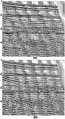 Figure 6.1-24 The CMP stacks after the model-based subtraction for multiple attenuation, which was implemented using filtered model traces. (a) First pass using multiple velocities V M1 and (b) second pass using multiple velocities V M2, as depicted in Figure 6.1-8b.


See also
- Periodicity of multiples
- Velocity discrimination between primaries and multiples
- Karhunen-Loeve transform
External links
| find literature about Modeling of multiples |