Derivation of AVO attributes by prestack amplitude inversion

Seismic Data Analysis

Series	Investigations in Geophysics
Author	Öz Yilmaz
DOI	http://dx.doi.org/10.1190/1.9781560801580
ISBN	ISBN 978-1-56080-094-1
Store	SEG Online Store

Following the prestack signal processing and prestack time migration designed for AVO analysis, prestack amplitude inversion is applied to the CRP gathers from prestack time migration. Whatever the basis for the AVO equations (Figure 11.2-22), derivation of the AVO attributes requires knowledge of the angle of incidence. This in turn requires, strictly, an estimated earth model in depth that can be used to trace rays associated with the CRP geometry. Figure 11.2-35 shows a velocity-depth model associated with the CRP stack shown in Figure 11.2-32. Often, the following procedure is adequate for a velocity-depth model estimation for the purpose of AVO analysis (models with horizontal layers):

1. Interpret a set of time horizons from the CRP stack (Figure 11.2-32).
2. Intersect the migration velocity field from step (g) of the prestack time migration sequence described above, which is equivalent to the rms velocity field associated with the vertical raypaths, with the time horizons from step (a) and create a set of horizon-consistent rms velocity profiles.
3. Perform Dix conversion of the rms velocity profiles to derive a set of interval velocity profiles.
4. Convert the time horizons from step (a) to depth horizons by using the interval velocity profiles from step (c) along image rays.
5. Combine the depth horizons from step (d) with the interval velocity profiles from step (c) and build a velocity-depth model as shown in Figure 11.2-35.

• 

  Figure 11.2-22  Framework for derivation of the various AVO equations in analysis of amplitude variation with offset.

• 

  Figure 11.2-32  Migration of the stack in Figure 11.2-31 using the rms velocity field derived from the velocity analysis of the CRP gathers as in Figure 11.2-28. The area within the rectangle corresponds approximately to the sections in Figures 11.2-41 and 11.2-42.

• 

  Figure 11.2-35  A velocity-depth model associated with the data as in Figure 11.2-32.

Before we proceed with prestack amplitude inversion to derive the AVO attributes, we first need to verify the existence of amplitude variation with offset on recorded data by modeling the amplitudes on a CRP gather coincident with a well location. Actually, we model a moveout-corrected CMP gather at the well location using a locally flat earth model, which is consistent with the earth model associated with the CRP gather. Figure 11.2-36 shows a sonic and a density log at a well location that coincides with the CMP location 1134 (Figure 11.2-32). By using the log curves and the S-wave velocity calculated from the mudrock relation (equation 42), compute the synthetic CMP gather associated with a horizontally layered earth model at the well location. Figure 11.2-37 shows a portion of the CRP gather from prestack time migration as in Figure 11.2-28 and the synthetic CMP gather computed by using the Zoeppritz equation for P-to-P reflection amplitudes associated with a horizontally layered earth model (Section L.5). Shown also in this figure is the angle of incidence within the same time window as for the CRP gather derived from the velocity-depth model in Figure 11.2-35. It is evident that given the offset range of 150-3050 m, the maximum angle of incidence at the target zone (3.1-3.3 s) is nearly 30 degrees. This means that the AVO attributes based on the Shuey approximation (equation 24) can be considered accurate.

A close-up view of the real CRP gather and the synthetic gather of Figure 11.2-37 at the reservoir zone is shown in Figure 11.2-38. Note that the amplitude variations in the two gathers are fairly consistent. In fact, examine in Figure 11.2-39 the amplitude variation with offset at three time levels that coincide with top-gas, top-oil, and top-water boundaries. We may draw two conclusions from the comparison of the real and modeled amplitudes as a function of offset shown in Figure 11.2-39. First, note that the Zoeppritz-modeled (red) and the best-fit actual (dotted green) amplitude variation with offset are in very good agreement — it appears that if you scale one AVO curve by a constant, you will get the other AVO curve. Second, the amplitudes do indeed vary with offset — there is a decrease in amplitude with increasing offset at the top-gas and top-water boundaries, and there is an increase in amplitudes with increasing offset at the top-oil boundary.

The top-gas AVO curve shown in Figure 11.2-39 extracted from the real CRP gather is consistent with the observations made by Rutherford and Williams who classified the AVO anomalies associated with a shale formation over a gas-bearing sand formation. A Class 1 AVO anomaly indicates a large positive P-to-P normal-incidence amplitude (large positive AVO intercept attribute value) and a marked decrease in amplitudes with increasing offset, with a possible phase change at large offsets. According to the Rutherford-Williams classification, the top-gas AVO curve in Figure 11.2-39 can be labeled as Class 1. A Class 2 AVO anomaly indicates a small positive P-to-P normal-incidence amplitude (small positive AVO intercept attribute value) and a marked decrease in amplitudes with increasing offset, with a possible phase change at small-to-moderate offsets. Finally, a Class 3 AVO anomaly indicates a large negative P-to-P normal-incidence amplitude (large negative AVO intercept attribute value) and a marked decrease in amplitudes with increasing offset, typically manifested as bright-spot anomalies.

• 

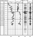  Figure 11.2-36  Log data measured at well location CRP 1134: (a) the sonic log, (b) the density log, (c) synthetic seismogram using a −90-degree phase-rotated band-limited wavelet (plotted at time 3.5 s), and (d) the reflectivity series computed from (a) and (b) and used in creating (c).

• 

  Figure 11.2-37  (a) A portion of the CRP gather 1134 at the well location as in Figure 11.2-29 within a time window that includes the reservoir zone between 3.1-3.3 s, (b) the synthetic CRP gather modeled by the Zoeppritz equation for P-to-P reflections, (c) the angle of incidence as a function of offset (the approximate angles at reservoir level are denoted at 3.1 s).

• 

  Figure 11.2-38  (b) A close-up portion of the CRP gather 1134 as in Figure 11.2-37a at the well location and at reservoir level, (b) the corresponding modeled CRP gather as in Figure 11.2-37b.

• 

  Figure 11.2-40  The stacks of the CRP data from prestack time migration as in Figure 11.2-28. The solid triangle denotes the well location at the surface, and the insertion below the well location is the synthetic equivalent of the sections shown. The dotted near-vertical line to the right is the well trajectory within the time gate corresponding to the portion of the sections shown.

Another AVO indicator is the difference between a near-angle stack (say, up to 15 degrees of angle of incidence as shown in Figure 11.2-37c) and a wide-angle stack (say, between 15-30 degrees of angles of incidence as shown in Figure 11.2-37c). If there were no amplitude variation with offset, there would not be a difference between the two sections shown in Figure 11.2-40, except for noise and residual moveout errors.

To calibrate the sections in Figure 11.2-40 to well data, compute the reflectivity series using the two log curves in Figure 11.2-36. Then, by using a zero-phase band-limited wavelet with a passband that corresponds to the signal band associated with the prestack time-migrated data (Figure 11.2-32), compute the zero-offset synthetic seismogram that contains primaries only. Insert the synthetic seismogram into the CRP stack at the well location as shown in Figure 11.2-40. Apply constant time shift and constant phase shift until a good match at the reservoir level is attained between the real and the synthetic data. In the present case, a constant time shift only, without a constant phase shift, was adequate to achieve a good match at the reservoir level.

See also

• Analysis of amplitude variation with offset
• Reflection and refraction
• Reflector curvature
• AVO equations
• Processing sequence for AVO analysis
• Interpretation of AVO attributes
• 3-D AVO analysis

External links

find literature about Derivation of AVO attributes by prestack amplitude inversion

References

- ↑ Rutherford and Williams (1989), Rutherford, S. R. and Williams, R. H., 1989, Amplitude-versus-offset variations in gas sands: Geophysics, 54, 680–688.