The problem of nonstationarity

Seismic Data Analysis

Series	Investigations in Geophysics
Author	Öz Yilmaz
DOI	http://dx.doi.org/10.1190/1.9781560801580
ISBN	ISBN 978-1-56080-094-1
Store	SEG Online Store

Figure 2.6-1 shows a CMP gather and its filtered versions before deconvolution. The filter scans show that there is signal between 10 to 40 Hz. Note that higher frequencies are confined to the shallower part of the gather. The same field record after spiking deconvolution is shown in Figure 2.6-2. Filter scans of the deconvolved record also are shown in this figure. A comparison of the records before and after deconvolution (Figures 2.6-1 and 2.6-2) demonstrates the effects of the process; in particular, compression of the wavelet and broadening of the spectrum. The input signal level above 40 Hz is relatively weaker than that below 40 Hz. Deconvolution has attempted to reduce the differences between the signal levels within different frequency bands by flattening the spectrum. The flattening, however, was more effective in the shallow part of the record than in the deeper part.

As discussed in gain applications and the convolutional model in the time domain, the source wavelet is not stationary — its shape and bandwidth change with traveltime (Figure 2.1-2). Specifically, attenuation of high frequencies in the wavelet increases as waves travel deeper in the subsurface. Although multiwindow deconvolution was used in this case (Figure 2.6-2), spectral flattening was not achieved over the entire length of the record because of the large degree of non-stationarity of the data. Nonstationarity is primarily the result of the effects of wavefront divergence and frequency attenuation.

The phenomenon of nonstationarity on stacked data is exemplified in Figure 2.6-3. Following a single-gate poststack spiking deconvolution, note that the average amplitude spectrum of the data does not indicate a flat spectrum (Figure 2.6-3b). Instead, the spectral behavior is similar to data with predictive deconvolution with a large prediction lag (Figure 2.6-3c). The strong reflector in the neighborhood of 2.5 s separates the zone with two different bandwidths — a broad-band signal zone above, and a relatively narrow-band zone below.

• 

  Figure 2.1-2  A seismic source wavelet after onset takes the form shown at top left. As the wavelet travels into the earth, the amplitude level drops (geometric spreading) and a loss of high frequencies occurs (frequency absorption).

• 

  Figure 2.6-1  A field record (far left panel) with its band-pass filtered versions.

• 

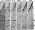  Figure 2.6-2  Spiking deconvolution applied to the field record in Figure 2.6-1 (far left panel), followed by application of a series of band-pass filters.

• 

  Figure 2.6-3  (a) A portion of a CMP-stacked section with its amplitude spectrum averaged over the CMP range (top) and autocorrelogram (bottom); (b) after time-invariant spiking deconvolution; and (c) after time-invariant predictive deconvolution with a prediction lag of 24 ms.

The usual approach to reduce nonstationarity is to apply processes designed to compensate for the effects wavefront divergence and frequency attenuation before deconvolution. Wavefront divergence is corrected for by applying a geometric spreading function (Gain applications). As yet, a method to compensate for attenuation has not been discussed. Attenuation is measured by a quantity called the quality factor Q. An infinite Q means that there is no attenuation. This factor can change in depth and in the lateral direction. If we had an analytic form for an attenuation function, then it would be easy to compensate for its effect. Several models for Q have been proposed. The constant-Q model is quite plausible and the easiest to deal with . However, the big problem of estimating Q from seismic data still remains. If a reliable Q value is available, say from borehole measurements, then, as will be discussed later in this section, inverse Q filtering can be applied to data to compensate for the frequency attenuation.

See also

• Time-variant deconvolution
• Time-variant spectral whitening
• Frequency-domain deconvolution
• Inverse Q filtering
• Deconvolution strategies
• Exercises
• Mathematical foundation of deconvolution

External links

find literature about The problem of nonstationarity

References

- ↑ Kjartansson, 1979, Kjartansson, E., 1979, Constant Q-wave propagation and attenuation: J. Geophys. Res., 84, 4737–4748.