Introduction to compressed sensing

Compressed sensing (CS) is an emerging field of mathematics and engineering that challenges the conventional paradigms of digital data acquisition. Since the seminal publication of Candès et al. (2006), the field has developed a substantial academic literature and has provided the foundation for major innovations in medical imaging, astronomy, and digital photography. Although CS is very mathematical, it can be conceptually intuitive. This tutorial provides a brief introduction to CS concepts through simple examples and interactive figures in an accompanying Jupyter notebook at github.com/seg/tutorials.

Overview

Many signals have an inherently low-dimensional structure, meaning all the information can be compressed into relatively few coefficients. As a simple example, consider the signal $x(t)=A\sin(ft+\phi )$, which is constructed with only three pieces of information: the amplitude A, the frequency f, and the phase $\phi$. Measuring this signal by using conventional acquisition requires sampling the entire duration of the signal at a rate of at least 2f, which results in 600 samples for a 10-s, 30-Hz signal. Why did we collect 600 samples of data when we require only three pieces of information? This is the fundamental question that compressed sensing is asking. In a field with large data-acquisition costs, we should pay close attention to the answers.

To gain some basic intuition into CS, this tutorial demonstrates the compressed acquisition of the simple 1D signal, where $f_{1}=10Hz,f_{2}=40Hz,\phi _{1}={\frac {\phi }{5}}$ and $\phi _{2}={\frac {\pi }{9}}$:

$x(t)=50\sin(2\pi f_{1}t+\phi _{1})+100\sin(2\pi f_{2}t+\phi _{2})$

Sparsity

The first requirement for compressed sensing is the existence of a sparse signal representation. We need to know a priori that the signal we are acquiring has relatively few nonzero coefficients in some transform domain. That might seem like a heavy requirement, but fortunately, the field of data compression has found sparsifying transforms for many types of general signal classes. For example, the Fourier transform compresses harmonic signals, the wavelet transform compresses images, and curvelets sparsify seismic data. In our simple example, let us assume that we know the signal has harmonic content and is therefore sparse in the Fourier domain.

Sampling

Let us make the jump from data compression to compressed sensing, in which we will try to exploit the compressibility of our signal directly during acquisition. Let us look first at the limitations of uniform sampling and then move on to other sampling methods.

For decades, uniform sampling has been the engineered data-acquisition strategy, in which Shannon-Nyquist theory says we can represent our signal uniquely by sampling at a rate of at least twice the highest frequency. Considering that our test signal can be reduced to only two samples of information, we are grossly oversampling, but we run into trouble with fewer samples. Figure 1 show the result of trying to reconstruct the test signal from fivefold undersampling below the Nyquist rate. As a result of the subsampling, we have introduced new frequency components called aliases. When we try to reconstruct our test signal, we are filling the gaps between samples incorrectly.

Fundamentally, aliasing occurs when multiple signals have the same value at every sample, which creates ambiguity to what the true signal is. When we violate the Nyquist rate, we no longer can fill gaps between data samples uniquely. Figure 2a demonstrates two aliased signals; the signals are identical at every sample point.

• 

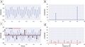  Figure 1. (a) Simple test-signal time series. (b) Amplitude half-spectra of the test signal. (c) Sampling and reconstruction of the test signal using fivefold regular subsampling. (d) Aliased spectrum of the fivefold regularly subsampled test signal.

• 

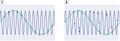  Figure 2. (a) Demonstration of aliasing caused by periodic sampling. (b) Breaking aliased signals using a random sample pattern.

• 

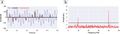  Figure 3. (a) Sampling and reconstruction using fivefold random undersampling. (b) Amplitude spectrum of fivefold random subsampling of the test signal. The threshold is shown for perfect signal reconstruction.

The problem is that both the signal and sampling pattern are periodic, which causes them to coherently interfere with each other. If our sampling pattern were aperiodic, it would be unlikely for different signals to have exactly the same value at every sample. The easiest way to break coherency is to use a random sampling pattern. Figure 2b shows that the aliased signals become distinguishable when we sample at random times.

We have shown that we can break aliasing patterns by random sampling, so let us return to the problem of subsampling our test signal. Note the differences in the Fourier spectrum (Figure 3a) compared with the aliased result we saw earlier. Since we broke the coherency of our sampling pattern, aliased signals have become random noise. We did not recover our signal (Figure 3b) because of the added noise. However, now that we have removed the ambiguity of aliasing, we can exactly reconstruct our signal through denoising techniques such as thresholding.

Recovery

The recovery stage of compressed sensing is the most challenging because it requires significant a priori knowledge of the signal. For our test signal, we can reconstruct the original signal fully by taking the two largest Fourier coefficients and renormalizing the signal energy. This requires prior knowledge of the number of nonzero coefficients in our signal or knowledge of an acceptable threshold value. In practice, recovery is often posed as an optimization problem in which we search for the smallest number of coefficients that can fit our sampled data within a given tolerance.

Seismic applications

This tutorial demonstrated CS concepts to a compressed acquisition of a simple signal, but how can we scale to seismic acquisition? We showed that for compressed sensing to be successful, we need

• a transform domain that can represent our data sparsely
• a sampling pattern that is incoherent in the transform domain
• a reconstruction method that promotes a priori knowledge about the signal sparsity

All of these are active fields of research in the seismic community. Curvelets have shown promise as a potential sparse representation of seismic data, and “low-rank” methods which exploit redundant structure in the midpoint-offset domain also are gaining traction with researchers.

Applying random sampling patterns is simple in theory, but in practice, it requires significant reengineering of the way we collect data. Seismic surveys are massive and use large vessels, streamer arrays, and precise logistics that all have been designed to collect data at regular intervals. Real-world random acquisition, although challenging, is a tractable problem, given adequate investment.

Confidence in the reconstruction is perhaps the largest hurdle in the uptake of CS methodology because it is difficult to impose an engineering specification on prior knowledge of signal sparsity or the rank of your data matrix. The a priori assumptions required for signal recovery are dependent on the local geology and carry a high level of uncertainty.

Simulations as well as synthetic resampling of seismic data have shown high signal-to-noise reconstructions with as much as tenfold subsampling. Although it is exciting, these are not blind experiments, and in many cases, they use knowledge of the true signal when defining reconstruction conditions. Compressed sensing has the potential to be a disruptive innovation in seismic acquisition, and it poses an interesting high-risk, high-reward engineering problem.

See also

• Bryan, K., and T. Leise, 2013, Making do with less: An introduction to compressed sensing: SIAM Review, 55, no. 3, 547–566, http://dx.doi.org/10.1137/110837681.
• Hennenfent, G., and F. J. Herrmann, 2008, Simply denoise: Wavefield reconstruction via jittered undersampling: Geophysics, 73, no. 3, V19–V28, http://dx.doi.org/10.1190/1.2841038.
• Mansour, H., H. Wason, T. T. Y. Lin, and F. J. Herrmann, 2012, Randomized marine acquisition with compressive sampling matrices: Geophysical Prospecting, 60, no. 4, 648–662, http://dx.doi.org/10.1111/j.1365-2478.2012.01075.x.

External links

• Madagascar workflow - reproducible using Madagascar open-source software
• Corresponding author: Ben Bougher (ben.boughergmail.com), University of British Columbia

find literature about Introduction to compressed sensing

References

- ↑ Candès, E. J., J. K. Romberg, and T. Tao, 2006, Stable signal recovery from incomplete and inaccurate measurements: Communications on Pure and Applied Mathematics, 59, no. 8, 1207–1223, http://dx.doi.org/10.1002/cpa.20124