Instantaneous attributes/en
 | |
| Series | Investigations in Geophysics |
|---|---|
| Author | Öz Yilmaz |
| DOI | http://dx.doi.org/10.1190/1.9781560801580 |
| ISBN | ISBN 978-1-56080-094-1 |
| Store | SEG Online Store |
Aside from the AVO attributes, the instantaneous attributes can be helpful in inferring reservoir parameters. When considered as an analytic signal (in the mathematical sense), a seismic trace can be expressed as a complex function [1]. An analytic signal is expressed by a time-dependent complex variable u(t)
Failed to parse (SVG (MathML can be enabled via browser plugin): Invalid response ("Math extension cannot connect to Restbase.") from server "https://en.wikipedia.org/api/rest_v1/":): u(t)=x(t)+iy(t), ( )
where x(t) is the recorded trace itself and y(t) is its quadrature. The quadrature is a 90-degree phase-shifted version of the recorded trace. It is obtained by taking the Hilbert transform of x(t) [2]
Failed to parse (SVG (MathML can be enabled via browser plugin): Invalid response ("Math extension cannot connect to Restbase.") from server "https://en.wikipedia.org/api/rest_v1/":): y(t)=\frac{1}{\pi t}*x(t). ( )
When substituted into equation (57), we have
Failed to parse (SVG (MathML can be enabled via browser plugin): Invalid response ("Math extension cannot connect to Restbase.") from server "https://en.wikipedia.org/api/rest_v1/":): u(t)=x(t)\left[\delta(t)+i\frac{1}{\pi t}\right]*x(t). ( )
Thus, to get the analytic signal u(t) for a seismic trace x(t), the complex operator [δ(t) + i/πt] is applied to the trace. When analyzed in the Fourier transform domain, this operator is zero for negative frequencies. Therefore, the complex trace u(t) does not contain negative frequency components.
Once u(t) is computed, it can be expressed in polar form as
Failed to parse (SVG (MathML can be enabled via browser plugin): Invalid response ("Math extension cannot connect to Restbase.") from server "https://en.wikipedia.org/api/rest_v1/":): u(t)=R(t)\exp[i\phi(t)], ( )
where
Failed to parse (SVG (MathML can be enabled via browser plugin): Invalid response ("Math extension cannot connect to Restbase.") from server "https://en.wikipedia.org/api/rest_v1/":): R(t)=\sqrt{x^2(t)+y^2(t)} ( )
and
Failed to parse (SVG (MathML can be enabled via browser plugin): Invalid response ("Math extension cannot connect to Restbase.") from server "https://en.wikipedia.org/api/rest_v1/":): \phi(t)=\arctan\frac{y(t)}{x(t)}. ( )
R(t) represents instantaneous amplitude and ϕ(t) represents instantaneous phase at time t. In practice, instantaneous phase is computed by first taking the logarithm of both sides of equation (60)
Failed to parse (SVG (MathML can be enabled via browser plugin): Invalid response ("Math extension cannot connect to Restbase.") from server "https://en.wikipedia.org/api/rest_v1/":): \ln u(t) = \ln R(t) + i \phi(t) ( )
and extracting the imaginary part
Failed to parse (SVG (MathML can be enabled via browser plugin): Invalid response ("Math extension cannot connect to Restbase.") from server "https://en.wikipedia.org/api/rest_v1/":): \phi(t) = {\rm Im}[\ln u(t)], ( )
where Im denotes imaginary.
The instantaneous frequency ω(t) is the temporal rate of change of the instantaneous phase function
Failed to parse (SVG (MathML can be enabled via browser plugin): Invalid response ("Math extension cannot connect to Restbase.") from server "https://en.wikipedia.org/api/rest_v1/":): \omega(t)=\frac{d\phi(t)}{dt}. ( )
When the derivative of equation (63) is taken with respect to time,
Failed to parse (SVG (MathML can be enabled via browser plugin): Invalid response ("Math extension cannot connect to Restbase.") from server "https://en.wikipedia.org/api/rest_v1/":): \frac{d\phi(t)}{dt}={\rm Im} \left[\frac{1}{u(t)}\frac{du(t)}{dt}\right]. ( )
For practical implementation, equation (64b) is written as the difference equation
Failed to parse (SVG (MathML can be enabled via browser plugin): Invalid response ("Math extension cannot connect to Restbase.") from server "https://en.wikipedia.org/api/rest_v1/":): \omega_t=\frac{2}{\Delta t}{\rm Im} \left[\frac{u_t-u_{t-\Delta t}} {u_t+u_{t-\Delta t}}\right]. ()
The instantaneous amplitude measures the reflectivity strength, which is proportional to the square root of the total energy of the seismic signal at an instant of time. The instantaneous phase is used to emphasize the continuity of events on a seismic section. The temporal rate of change of the instantaneous phase is the instantaneous frequency. The instantaneous frequency may have a high degree of variation, which may be related to stratigraphy. However, it also may be difficult to interpret all this variation. Therefore, the instantaneous frequency values often are smoothed in time.
The instantaneous measurements that are related to an analytic signal are associated with an instant of time, rather than an average over a time interval. These measurements are reliable when the seismic signal is recorded and processed so that the CMP stack closely represents the subsurface. In other words, to deduce any stratigraphic meaning from the seismic data before estimating the instantaneous parameters, the amplitude and frequency content of the seismic signal must be preserved in each processing step. Any variation in the shape of the basic waveform that is not attributable to the subsurface geology must be eliminated. Multiples and all types of random noise limit the reliability of the results.
Reflectivity strength is an effective tool to identify bright and dim spots. Phase information is useful in delineating such interesting features as pinchouts, faults, onlaps, and prograding reflections. Instantaneous frequency information can help to identify condensate reservoirs and gas reservoirs, which tend to attenuate high frequencies.
Instantaneous attributes often are displayed in color for interpretation. Figure 11.3-32 shows the instantaneous attributes that correspond to the seismic section in Figure 11.3-1. The seismic data are displayed on top of the attributes as wiggle traces. Note the distinctive anomaly on the instantaneous amplitude section and enhancement of the continuity of reflections on the instantaneous phase section.
-
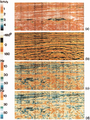 Figure 11.3-32 Instantaneous attributes derived from the stacked section in Figure 11.3-1: (a) reflectivity strength, (b) phase, (c) frequency, and (d) smoothed frequency.
 -
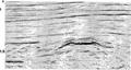 Figure 11.3-1 A portion of a CMP stack containing a bright spot.


References
See also
- Acoustic impedance estimation
- Synthetic sonic logs
- Processing sequence for acoustic impedance estimation
- Derivation of acoustic impedance attribute
- 3-D acoustic impedance estimation
External links
| find literature about Instantaneous attributes/en |

|

|

|

|

|

|

|