Fundamentals of signal processing exercises

Seismic Data Analysis

Series	Investigations in Geophysics
Author	Öz Yilmaz
DOI	http://dx.doi.org/10.1190/1.9781560801580
ISBN	ISBN 978-1-56080-094-1
Store	SEG Online Store

Exercise 1-1. Refer to Figure 1.E-1. Using equation (2), compute the alias frequencies at 4- and 8-ms sampling intervals for the three frequency components — A, B and C from the amplitude spectrum of the 2-ms time series. Confirm the results of your computation by the amplitude spectra.

$ {{f}_{a}}=\left|2m\,{{f}_{N}}-{{f}_{s}}\right|, $

(2)

Exercise 1-2. Using the hyperbolic traveltime equation, compute the average velocity down to reflector A in Figure 1.3-8. Assume a constant velocity between A and the surface. The required information about Record 8 is in Table 1-13.

Exercise 1-3. What is the dispersive event C in Figure 1.3-8?

Exercise 1-4. Refer to the walk-away noise test record in Figure 1.3-19. Measure the phase velocity (Δx/Δt) of the ground-roll energy at location A₁. Also measure the dominant frequency at the same location. Then, estimate the dominant wavelength (velocity/dominant frequency) of the ground roll. The receiver array length needed to suppress this energy in the field should be equal to or greater than the longest noise wavelength. The required information about Record 19 that you need for your computations is in Table 1-13.

Exercise 1-5. Measure the group velocity (x/t) of ground-roll energy A in Figure 1.3-25. The required information for Record 25 is in Table 1-13.

Exercise 1-6. Refer to the shot record in Figure 1.3-27. The near-offset 28 channels were recorded using a 50-m group interval. What is the group interval for the remaining 64 channels? The required information for Record 27 is in Table 1-13.

Exercise 1-7. What is event A in Figure 1.3-29? Are events C, D, and E multiples of B?

Exercise 1-8. Refer to Figure 1.3-30. Compute the water velocity using both the direct arrivals A and the water-bottom reflection B. Use one-way time for A and two-way time for B. The required information for Record 30 is in Table 1-13.

Exercise 1-9. Identify events A, B, C, D, E, and F in Figure 1.3-33.

Exercise 1-10. Identify events A, B, C, D, and E in Figure 1.3-34.

Exercise 1-11. Gain application involves multiplying the gain function with the seismic trace (Figure 1.4-8). Use the appropriate entry in Table A-1 to describe the effect of the gain application in the frequency domain.

Exercise 1-12. From Figure 1.E-2, identify the common-shot and common-midpoint gathers.

Exercise 1-13. Use equation (12) to compute fold n_f for each of the following recording geometries:

Number of Channels	Shot Spacing, m	Receiver Spacing, m
240	25	25
240	50	25
240	100	25
240	25	50

$ {n_{f}}={\frac {{n_{g}}\Delta g}{2\Delta s}}, $

(12)

Exercise 1-14. Consider the recording geometry in Figure 1.5-8. Sketch the traveltime curves on a common-shot gather associated with point scatterers (a) beneath the cable, (b) behind, and (c) in front of the cable. Assume all scatterers are on the plane of recording.

Exercise 1-15. Suppose that the shot associated with gather 1 in Figure 1.5-10 is missing. Identify the midpoints that are affected by this missing shot; that is, the midpoints with a lower fold of coverage. Suppose the receiver associated with gather 2 in Figure 1.5-10 is missing. Identify the midpoints that are affected by this.

Exercise 1-16. Prove the shifting, scaling, and differentiation rules applied to the Fourier transform of a function given by the entires (1), (2), and (3) in Table A-1.

Figures and tables

• 
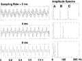  Figure 1.E-1  A signal with three frequency components, A, B, and C, sampled at three different rates, 2, 4, and 8 ms. Frequency aliasing occurs at coarser sampling intervals.
• 
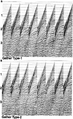  Figure 1.E-2  A field data set displayed in two different domains — common-shot and common-midpoint (see Exercise 1-12).
• 
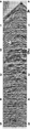  Figure 1.3-8  Worldwide assortment record 8.
• 
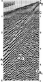  Figure 1.3-19  Worldwide assortment record 19.
• 
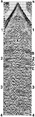  Figure 1.3-25  Worldwide assortment record 25.
• 
  Figure 1.3-27  Worldwide assortment record 27. Identify the direct wave on this record.
• 
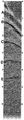  Figure 1.3-29  Worldwide assortment record 29.
• 
  Figure 1.3-30  Worldwide assortment record 30.
• 
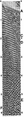  Figure 1.3-33  Worldwide assortment record 33.
• 
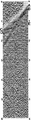  Figure 1.3-34  Worldwide assortment record 34.
• 
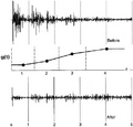  Figure 1.4-8  Gain is a time-variant scaling defined by a function, g(t). Based on some criteria, this function is defined at the time samples (shown by solid circles) that are usually at the center of specified time gates along the trace as indicated by 1, 2, 3, and 4. Gain application simply involves multiplying g(t) by the input trace amplitudes.
• 
  Figure 1.5-8  (a) Seismic data acquisition is done in shot-receiver (s, g) coordinates. The raypaths are associated with a planar horizontal reflector from a shot point (indicated by the solid circles) to several receiver locations (indicated by the triangles). The processing coordinates, midpoint-(half) offset, (y, h) are defined in terms of (s, g): y = (g + s)/2, h = (g − s)/2. The shot axis here points opposite the profiling direction, which is to the left. On a flat reflector, the subsurface is sampled by reflection points which span a length that is equal to half the cable length. (b) Seismic data processing is done in midpoint-offset (y, h) coordinates. The raypaths are associated with a single CMP gather at midpoint location M. A CMP gather is identical to a CDP gather if the depth point were on a horizontally flat reflector and if the medium above were horizontally layered.
• 
  Figure 1.5-10  (a) A hypothetical stacking chart (adapted from ). Each dot represents a single trace with the time axis perpendicular to the plane of the page. Shot-geophone (s, g), and midpoint-offset (y, h) coordinates are superimposed with the (y, h) plane rotated 45 degrees with respect to the (s, g) plane. Here, (1) is a common-shot gather, (2) is a common-receiver gather, (3) is a CMP gather, (4) is a common-offset section, and (5) is a CMP-stacked section. The remaining notation is defined in the text. (b) Raypaths associated with (1) a common-shot gather, (2) a common-receiver gather, (3) a CMP gather, and (4) a common-offset section. Solid triangles denote receiver locations and solid circles denote shot locations, x is the effective cable length — the difference between the maximum and minimum offsets, E denotes a midpoint and E’ denotes a depth point on a flat reflector.

Table 1-13. Parameter index of a worldwide assortment of common-shot gathers.

Record Number	Area	Number of Samples per Trace	Number of Traces	Sampling Interval, ms	Trace Interval, ft or m	Inner Offset, ft or m	Source
1	South Texas	1,275	48	4	330 ft	990 ft	V
2	West Texas	1,025	120	4	100 ft	400 ft	V
3*	Louisiana	1,500	24	4	340 ft	340 ft	D
4	Turkey	1,275	48	4	100 m	250 m	V
5	South America	3,000	48	2	100 m	200 m	D
6	Far East	1,250	48	4	100 m	150 m	D
7	South America	2,600	48	2	100 m	300 m	V
8	Central America	1,300	96	4	50 m	100 m	D
9	Alaska	1,000	96	4	220 ft	990 ft	V
10	North Africa	1,325	120	4	25 m	300 m	V
11	Alaska	1,000	96	4	220 ft	990 ft	V
12	Mississippi	1,275	48	4	330 ft	990 ft	V
13	Offshore Texas	2,025	48	4	220 ft	875 ft	A
14	Offshore Texas	1,525	48	4	220 ft	690 ft	P
15	Offshore Canada	2,500	48	2	25 m	360 m	A
16	South America	1,275	48	4	25 m	233 m	A
17	South America	2,000	48	4	50 m	250 m	A
18	Offshore Louisiana	1,500	120	4	82 ft	716 ft	A
19	Turkey	1,250	216	4	10 m	50 m	D
20	South Aleutians	2,025	120	4	82 ft	921 ft	A
21	Denver Basin	1,550	48	2	220 ft	220 ft	V
22	Williston Basin	1,550	48	2	110 ft	110 ft	V
23	San Juaquin Basin	1,550	48	2	220 ft	220 ft	V
24	Arctic	3,000	48	2	220 ft	220 ft	S
25	Alberta	2,000	96	2	50 m	50 m	D
26	Alberta	1,500	48	2	67 m	67 m	D
27	Canada	1,791	92	4	50 m	200 m	A
28	Canada	2,500	48	2	25 m	300 m	A
29	Offshore Spain	2,000	48	4	50 m	250 m	M
30	Offshore Crete	2,125	96	4	25 m	230 m	A
31	North Sea	1,550	96	4	25 m	228 m	A
32	North Sea	1,550	96	4	25 m	178 m	A
33	North Sea	1,625	96	4	25 m	200 m	A
34	Celtic Sea	1,500	60	4	50 m	253 m	A
35	Denmark	2,500	52	2	100 m	100 m	D
36	Middle East	1,024	48	4	50 m	250 m	V
37	Turkey	1,000	48	4	75 m	187 m	V
38	North Africa	2,500	60	2	100 m	100 m	V
39	Middle East	2,500	60	2	50 m	100 m	G
40	West Africa	2,600	96	2	30 m	120 m	D

*Analog recording. V: vibroseis, D: dynamite, A: Air gun, P: Aquapulse, M: Maxipulse, G: Geoflex, S: Aquaseis. All vibroseis records have been correlated. Aquapulse and Maxipulse are registered trademarks of Western Geophysical Company of America. Aquaseis and Geoflex are registered trademarks of Imperial Chemical Industries.

Table A-1. Fourier transform theorems (Bracewell, 1965).

Operation	Time Domain	Frequency Domain
(1) Shifting	x(t − τ)	exp(−iωτ)X(ω)
(2) Scaling	x(at)	$ {{\left|a\right|}^{-1}}X\left({\omega }/{a}\;\right) $
(3) Differentiation	dx(t)/dt	iωX(ω)
(4) Addition	f(t) + x(t)	F(ω) + X(ω)
(5) Multiplication	f(t) x(t)	F(ω)* X(ω)
(6) Convolution	f(t)* x(t)	F(ω) X(ω)
(7) Autocorrelation	x(t)* x(−t)	$ {{\left|X\left(\omega \right)\right|}^{2}} $
(8) Parseval’s theorem	$ \int {{\left|x\left(t\right)\right|}^{2}}\ dt $	$ \int {{\left|X\left(\omega \right)\right|}^{2}}\ d\omega $

* denotes convolution.

See also

• Introduction to fundamentals of signal processing
• The 1-D Fourier transform
• The 2-D Fourier transform
• Worldwide assortment of shot records
• Gain applications
• Basic data processing sequence
• A mathematical review of the Fourier transform

External links

find literature about Fundamentals of signal processing exercises