Dip-moveout correction in practice

Seismic Data Analysis

Series	Investigations in Geophysics
Author	Öz Yilmaz
DOI	http://dx.doi.org/10.1190/1.9781560801580
ISBN	ISBN 978-1-56080-094-1
Store	SEG Online Store

Results of the previous section suggest the general DMO processing sequence shown in Figure 5.2-1.

1. Perform velocity analysis at sparse intervals and pick just a few velocity functions with minimal dip effects.
2. Apply NMO correction using the these flat-event velocities.
3. Sort data to common-offset sections, apply DMO correction and sort back to CMP gathers.
4. Apply inverse NMO correction using the flat-event velocities from step (a).
5. Perform velocity analysis at frequent intervals as needed to derive an optimum stacking velocity field.
6. Apply NMO correction using the optimum stacking velocity field.
7. Stack the data and migrate using an edited and appropriately smoothed version of the optimum stacking velocity field.

Note that this processing sequence is similar to the sequence for residual statics corrections described in Figure 3.3-12. Both residual statics and DMO corrections are followed by a revision of velocities so as to get the most out of these corrections during stacking. In this section, we shall apply the sequence outlined above to two common cases of conflicting dips with different stacking velocities — salt flanks and fault planes.

• 
  Figure 3.3-12  Processing flowchart with residual statics corrections.
• 
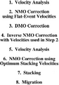  Figure 5.2-1  DMO processing flowchart.

See also

• Introduction to dip-moveout correction and prestack migration
• Principles of dip-moveout correction
• Prestack time migration
• Migration velocity analysis
• Exercises
• Topics in Dip-Moveout Correction and Prestack Time Migration

External links

find literature about Dip-moveout correction in practice